Model Development Typical Workflow on the C3 Agentic AI Platform
An example of the typical model development workflow on the C3 Agentic AI Platform is provided below. As a starting point for this example, we will assume that as an input to this step, we have a constructed a c3.Data instance that contains the data we wish to use for model training and testing. For the use case in this example, we will use labelled network flow data and attempt to predict when there was a DDoS attack occurring on the network.
df = c3.Data.read_csv('local://{Path_to_dataset}.csv')
y = df['Label']
X = df.drop(columns=['Label'], axis=1)Building blocks - MlPipes
MlPipes serve as the building blocks for arbitrarily complex machine learning pipelines. For details on MlPipes, see Machine Learning Pipes on the C3 Agentic AI Platform.
To continue with the above example, import any Python libraries that we might like to use for our experimentation.
from sklearn.ensemble import GradientBoostingClassifier, RandomForestClassifier
from sklearn.preprocessing import StandardScaler
Next, the entry point for the machine learning pipeline authoring framework in the C3 Agentic AI Platform is c3.MlPipeline.Authoring. We instantiate this variable and can use the .convert() method to translate native sklearn estimators into MlPipes, which can be used to construct production-ready MlPipelines. For details on platform-provided MlPipes, see Machine Learning Pipes on the C3 Agentic AI Platform.
While in this example we're using platform-provided building blocks, we could just as easily use our own machine learning estimator implemented purely in Python using the libraries of our choice. See Author Custom Machine Learning Pipes in Native Python - MlLambdaPipe Tutorial and Author Custom Machine Learning Pipes in Native Python - MlDynamicPipe Tutorial for detailed tutorials.
Use the code snippet below to instantiate c3.MlPipeline.Authoring for this example.
mla = c3.MlPipeline.Authoring

ss = StandardScaler()
ss_pipe = mla.convert(ss, spec=c3.SklearnLikeConvertSpec(keepInputColumnIndices=True))

clf = RandomForestClassifier(random_state=0, max_depth=5, n_estimators=20)
clf_pipe = mla.convert(clf, spec=c3.SklearnLikeConvertSpec(processFunc='predict'))
Additionally, using the code snippet above:
- We can set hyperparameters for our estimators in the native objects' constructor
- We can pass in additional specification corresponding to our estimator type:
SklearnLikeConvertSpec. In this specification, we can add arguments likeprocessFunc, which defines the function called through the underlying estimator when we callprocess. In our case, we have set it topredict.
Assemble MlPipeline
Now that we have individual pipes instantiated, we can connect them together in the form of an MlPipeline. The C3 Agentic AI Platform offers a versatile and scalable pipeline authoring framework that allows constructing arbitrarily complex productionizable workflows for machine learning. In the example below, we use the MlPipes created previously to author an MlPipeline.
X_input, y_input = mla.var(), mla.var()
accuracy_metric = c3.MlAccuracyMetric()
ss_out = ss_pipe(X_input)
y_output = clf_pipe(ss_out, y_input)
accuracy_out = accuracy_metric(y_input, y_output)

pipeline = mla.pipeline(
    x={'Features': X_input},
    y={'Label': y_input},
    out={'Predictions': y_output},
    scores={"Scores": accuracy_out}
)
X_input and y_input act as input placeholder variables and are used to begin constructing the graph representing this simple machine learning workflow. The intermediate variables can be passed through the intermediate MlPipes and MlScoringMetrics eventually arriving at the terminal placeholder variables y_output and accuracy_out. Finally, to construct the pipeline, we pass dictionaries labelling the inputs and outputs of our machine learning pipeline and the authoring framework takes the responsibility of creating the full MlPipeline DAG.
This graph can be visualized as shown below.
pipeline.visualize()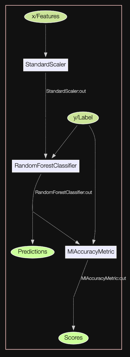
Since we have defined this pipeline using placeholder variables, this pipeline can directly be used to serve production predictions where the data for features x and label y are coming from databases. The exact pipeline you are using to experiment with using Pandas DataFrames or C3 AI Datasets can be used to serve production predictions, where the data is being materialized from databases and predictions are persisted back into databases.
Train the MlPipeline
Now we can pass our training data (instances of c3.Data) through the MlPipeline we have authored above. Note that by default training will be performed asynchronously server-side. Therefore, for retrieving the trained pipeline, we must call .result() on the MlOperationRun. See Author Machine Learning Pipelines - MlPipeline Tutorial for details.
pipeline_trained = pipeline.train(
    x={'Features': X_train},
    y={'Label': y_train}
).result()Generate predictions
Similar to training, we can generate predictions from our trained pipeline by calling the .process() method on the pipeline and passing in the dat we would like to use to generate predictions (instances of c3.Data). This operation will also run asynchronously server-side by default. Therefore, for retrieving the predictions, we must call .result() on the MlOperationRun.
See Author Machine Learning Pipelines - MlPipeline Tutorial for details.
predictions = pipeline_trained.process(
    x={'Features': X_train}
).result()
To retrieve the resulting prediction data (instance of c3.Data), we access the predictions based on the key of the pipeline output.
predictions['Predictions']| 0 | |
|---|---|
| 0 | 2 |
| 1 | 0 |
| 2 | 3 |
| 3 | 0 |
| 4 | 2 |
| ... | ... |
| 100 | 0 |
| 101 | 1 |
| 102 | 1 |
| 103 | 1 |
| 104 | 0 |
105 rows × 1 columns
Score output of pipeline
Since we had added the MlAccuracyMetric scoring metric to our pipeline, we can generate scores by passing in a dataset we’d like to score. In the code snippet below, we are computing the accuracy of our trained pipeline on the training dataset and accessing the result by using the key we used while authoring the scoring output of the pipeline.
score_output = pipeline_trained.score(x={'Features': X_train},
                                      y={'Label': y_train}).result()
score_output['Scores']0.9993291011854656This operation will also run asynchronously server-side by default. Therefore, for retrieving the predictions, we must call .result() on the MlOperationRun. See Author Machine Learning Pipelines - MlPipeline Tutorial for details.
Interpret pipeline and generate artifacts
Just as we have attached scoring metrics to our pipeline above, we can also attach interpreters to our pipeline. This allows us to call interpret() on the pipeline and generate artifacts for our trained machine learning estimators. See Interpretability Deep Dive - ShapInterpreter Authoring and Execution Tutorial for details.
Hyperparameter Optimization (HPO)
We instantiated our native sklearn RandomForestClassifier with certain hyperparameters. To perform a search over hyperparameters, we can simply modify the clf_pipe we created above and pass a dictionary of hyperparameter search spaces to the .withHyperparamSpaces() method.
clf = RandomForestClassifier()
clf_pipe = mla.convert(clf, spec=c3.SklearnLikeConvertSpec(processFunc='predict'))

clf_param_spaces = {'criterion': c3.Hp.ParamSpace.Categorical.fromValues(['gini', 'entropy']),
                    'max_depth': c3.Hp.ParamSpace.Categorical.fromValues([1, 3, 7])}

clf_pipe = clf_pipe.withHyperparamSpaces(clf_param_spaces)
We author the pipeline in the exact same way:
X_input, y_input = mla.var(), mla.var()
accuracy_metric = c3.MlAccuracyMetric()
ss_out = ss_pipe(X_input)
y_output = clf_pipe(ss_out, y_input)
accuracy_out = accuracy_metric(y_input, y_output)

pipeline = mla.pipeline(
    x={'Features': X_input},
    y={'Label': y_input},
    out={'Predictions': y_output},
    scores={"Accuracy": accuracy_out}
)
We can set which search algorithm we’d like to use. For a list all supported hyperparameter search algorithms, see Hyperparameter Optimization at Scale - HPO Tutorial.
my_optuna_search_algo = c3.Hpo.OptunaSearch(algorithm='Grid')We also set the cross-validation technique we’d like to use. For a list of all supported cross-validation techniques please refer to the detailed Hyperparameter Optimization at Scale - HPO Tutorial.
val_tech = c3.MlSplit.RandomHoldout(validationSize=0.1)Now we can put the search algorithm and validation technique together in an Hpo.Spec along with additional options for the distributed hyperparameter optimization run.
hpo_spec = c3.Hpo.Spec(validationTechnique=val_tech,
                       algorithm=my_optuna_search_algo,
                       maxTrials=4,
                       maxConcurrentTrials=2,
                       hpoMetric='Accuracy',
                       experimentName='My_Unique_Hpo_Name').withDefaults()
Now we can slightly modify the code we used above to train our pipeline, and pass in our constructed Hpo.Spec. The pipeline will implicitly do the search for the optimal hyperparameter combination as specified earlier. Once found, it will re-train the pipeline with these optimal hyperparameters on the whole input data.
train_run = pipeline.train(
    x={'Features': X_train},
    y={'Label': y_train},
    spec=c3.MlOperationSpec(hpoSpec=hpo_spec)
)
Now when we retrieve our final trained pipeline, it will be the pipeline with the best hyperparameters found during the search trained on the entire input dataset.
trained_pipeline = train_run.result()For a detailed walk-through of the hyperparameter optimization workflow pertaining to experiment tracking, inspection and debugging, see Hyperparameter Optimization at Scale - HPO Tutorial.
Cancel a MlOperationRun
To cancel a MlOperationRun, use MlOperationRun().run.cancel().