XGBoost Regression
Train an XGBoost regression model that can predict continuous values in Visual Notebooks. XGBoost is a popular and highly efficient gradient boosting algorithm.
Configuration
| Field | Description |
|---|---|
| Name | Name of the node A user-specified node name displayed in the workspace, both on the node and in the dataframe as a tab. |
| Select Column with Labels | The column the XGBoost regressor should predict Select a column from the dropdown menu. This column contains the values that the model should be able to predict after training. |
Select Features
| Field | Description |
|---|---|
| Select Features | Features to train the model with Use all columns as features, or select specific columns using the dropdown menu. Columns selected as features are used to train the model. |
| Select optional timeseries column | Timeseries column If there is a timeseries column in your data, check the box in this field and select the timeseries column from the auto-populated dropdown menu. Timeseries information is used when splitting the data into separate train, validation, and test datasets. |
Test and Validation Settings
When training models, data is split into multiple components. The bulk of the data is used for training and validation, while a small portion is set aside for testing. The fields in this section determine what percentage of the data is used for training, how the data is used during the training process, and the strategy used to split the data.
| Field | Description |
|---|---|
| Select test and validation method | Test and train method Select Train-validation-split to split the dataset into separate train, validation, and test datasets. Select Cross-validation to split the data into a specified number of subsets. During training, one subgroup is used for testing and validation, while the other subgroups are used for training. The process is then repeated so each subgroup is used as the testing and validation group once. |
| Select percentage split | Data split percentage Move the slider to split the data into test, validation, and train datasets. If Cross-validation is selected in the Select test and validation method field, move the slider to split the data into a train dataset that will be divided into subgroups, and a separate testing dataset. The default split when using the cross-validation method is 80% train and 20% test. |
| Select number of cross-validation folds | Number of cross-validation subgroups Enter a number between 2 and 20. The data allocated for training is divided into the specified number of subgroups. |
Scorer and Stopping Conditions
By default, Visual Notebooks trains many models with different hyperparameter configurations, then ranks the models by performance. The fields in this section tell Visual Notebooks when to stop making new models. You can stop making models once the new models no longer substantially improve upon the existing models. Alternatively, you can stop making new models after a specified number of models have been trained or a certain amount of time has passed.
| Field | Description |
|---|---|
| The performance metric | The performance metric used to stop hyperparameter search Select Mean Residual Deviance, MSE, RMSE, MAE, or RMSLE. When training multiple models with different hyperparameter combinations, stop creating models when the new models fail to improve a specified performance metric. Performance metrics are always some sort of error. Errors measure how far off the predictions of the model are to the actual values. When the model predicts a value close to the actual, the error is small, and when the model predicts a value far from the actual, the error is large. Here is an overview of these error metrics: MSE (Mean Squared Error): The average of the squared errors. MSE penalizes large errors harshly. RMSE (Root Mean Squared Error): The square root of MSE. RMSE also penalizes large errors harshly, and it is more interpretable by virtue of being measured in the same units as the labels and predictions. MAE (Mean Absolute Error): The average of the absolute errors. MAE does not penalize large errors as harshly as MSE or RMSE, for it does not square the errors. RMSLE (Root Mean Squared Logarithmic Error): The square root of the average of the log errors. RMSLE is primarily used when the ratio of the true value to the predicted value is the priority. Whereas all the other metrics above will penalize incorrect predictions made on large values more harshly, RMSLE does not. Thus, RMSLE is commonly used when there is a very large range of possible values . RMSLE is also famous for penalizing underestimates more harshly than overestimates and is thus used to rank models for siutations in which making an underestimate is worse than making an overestimate. This field is used in conjunction with the following two fields. |
| Does not improve by more than | The specific threshold used to stop hyperparameter search Select 0.1%, 0.01%, 0.001%, or 0.0001%. When training multiple models with different hyperparameter combinations, stop creating models when the new models fail to improve the specified performance metric by the given percentage. This field is used in conjunction with the fields directly above and below. |
| After the following number of consecutive training rounds | The criteria used to stop hyperparameter search Select a number between 2 and 10. When training multiple models with different hyperparameter combinations, stop creating models when the new models fail to improve the specified performance metric after the following number of consecutive training rounds. This field is used in conjunction with the two fields above. |
| A maximum # of models have been trialed | How many models to train Select 3, 5, 10, 20, 50, 100, 200, or 500. When training multiple models with different hyperparameter combinations, stop creating new models after a specified number of models are created. |
| A specified amount of training time passes | When to stop training new models Select 5 minutes, 10 minutes, 20 minutes, 30 minutes, 1 hour, 2 hours, 12 hours, or 24 hours. When training multiple models with different hyperparameter combinations, stop creating new models after a specified amount of time passes. |
Hyperparameters Search
As mentioned in the previous section, Visual Notebooks trains many different models with various hyperparameter combinations. The fields in this section determine the hyperparameter options used during training. Although you don't need to alter these fields to train a high-performing model, it is possible to explore different combinations.
Hyperparameters give you precise control over a model. You can use these to tell the model how quickly to learn, when to stop improving, and what to prioritize during the learning process. In general, the goal of changing the hyperparameters is to make the best possible model while avoiding overfitting. If a model is too closely aligned to the training data, it may be incapable of producing accurate predictions on unseen data.
| Field | Description |
|---|---|
| Hyperparameters Search | Train one model or multiple models Select Search to train multiple models with different hyperparameter combinations and then compare the models to find the best one. Select Fixed to train a single model with a fixed hyperparameter configuration. |
| Number of trees / estimators | The number of trees to build Enter an integer between 2 and 10,000. More trees create a more accurate model, but can lead to overfitting. Values between 50 and 200 are common. If you define a fixed model, the default is 50. |
| Maximum tree depth | The maximum number of levels in each tree Enter an integer between 1 and 100. Increasing the tree depth allows the model to fine-tune its performance, but may lead to overfitting. Values between 3 to 12 are common. If you define a fixed model, the default is 6. |
| Minimum child weight | The minimum number of data points in a leaf Enter an integer greater than or equal to 0. Increasing this value makes the model more generic, as it tells the model to stop splitting the tree if it will result in fewer than the specified number of data points in a leaf node. Values between 1 to 10 are common. If you define a fixed model, the default is 1. |
| Minimum split improvement (gamma) | Amount of improvement required to make an additional split of the tree Enter an integer greater than or equal to 0. Increasing this value makes the model more generic, as it tells the tree to stop splitting if it will result in an improvement less than the value of this field. Values of 0, 1, 5, and 10 are common. If you define a fixed model, the default is 0. |
| Column sample rate per tree | Amount of columns used during training by each tree Enter a number between 0 and 1. Each tree uses the given ratio of columns when training. Decreasing this value helps prevent individual columns from over-influencing the prediction. Values from 0.3 to 0.8 are common if the dataset has many columns, while values of 0.8 to 1 are common if the dataset has few columns. If you define a fixed model, the default is 1. |
| Row sample rate per tree | Amount of rows used during training by each tree Enter a number between 0 and 1. Each tree uses the given ratio of data when training. Decreasing this value helps prevent overfitting to accommodate outliers. Values from 0.8 to 1 are common. If you define a fixed model, the default is 1. |
| Learning rate | The learning speed Enter a number between 0 and 1. Decreasing this value improves performance, but increases training time. Values between 0.01 and 0.3 are common. If you define a fixed model, the default is 0.3. |
| L1 regularization (alpha) | Lasso regularization Enter a number greater than or equal to 0. Increasing this value discourages overfitting by penalizing overly complex models and removing some features. Values of 0, 1, 5, and 10 are common. If you define a fixed model, the default is 0. |
| L2 regularization (lambda) | Ridge regularization Enter a number greater than or equal to 0. Increasing this value discourages overfitting by penalizing overly complex models and lowering the importance of some features. Values of 0.01, 0.1, 1, and 10 are common. If you define a fixed model, the default is 1. |
Repeatability Seed
Random numbers are used throughout the training process for splitting the original dataset, splitting individual trees, and optimizing hyperparameters. Ex Machina uses one number, called a seed, to generate those random numbers. The field in this section allows you to enter a custom seed. If you enter a custom seed, you can enter that same custom seed at a later date to reproduce the results of the training.
| Field | Description |
|---|---|
| Seed | The number used throughout the AutoML process Select Random to use a random number, or select Custom to enter a specific integer. The seed is used to generate numbers used throughout the AutoML process. If you enter a custom seed, you can enter the same custom seed at a later date to get the same results. |
Prediction
The output of this node is each model's predictions on the training data. This section determines how the predictions are portrayed in the resulting dataframe.
| Field | Description |
|---|---|
| Prediction Column Name | The column name for the model's predictions Enter a name for the column that contains the selected model's predictions. Column names can contain alphanumeric characters and underscores, but cannot contain spaces. |
| Dataset Selection | Data used to display a model's predictions Select one of the following options: all data, train dataset, validation dataset, or test dataset. Visual Notebooks displays a selected model's predictions on the dataset selected with this field. |
| Include all columns | Whether to include all columns in the predictions table Select Toggle this to include all columns in the predictions table, including the columns that you did not use as features for the model. By default, only columns you selected as features will be included. |
Node Inputs/Outputs
| Input | A Visual Notebooks dataframe |
|---|---|
| Output | A dataframe with predictions on the training data |
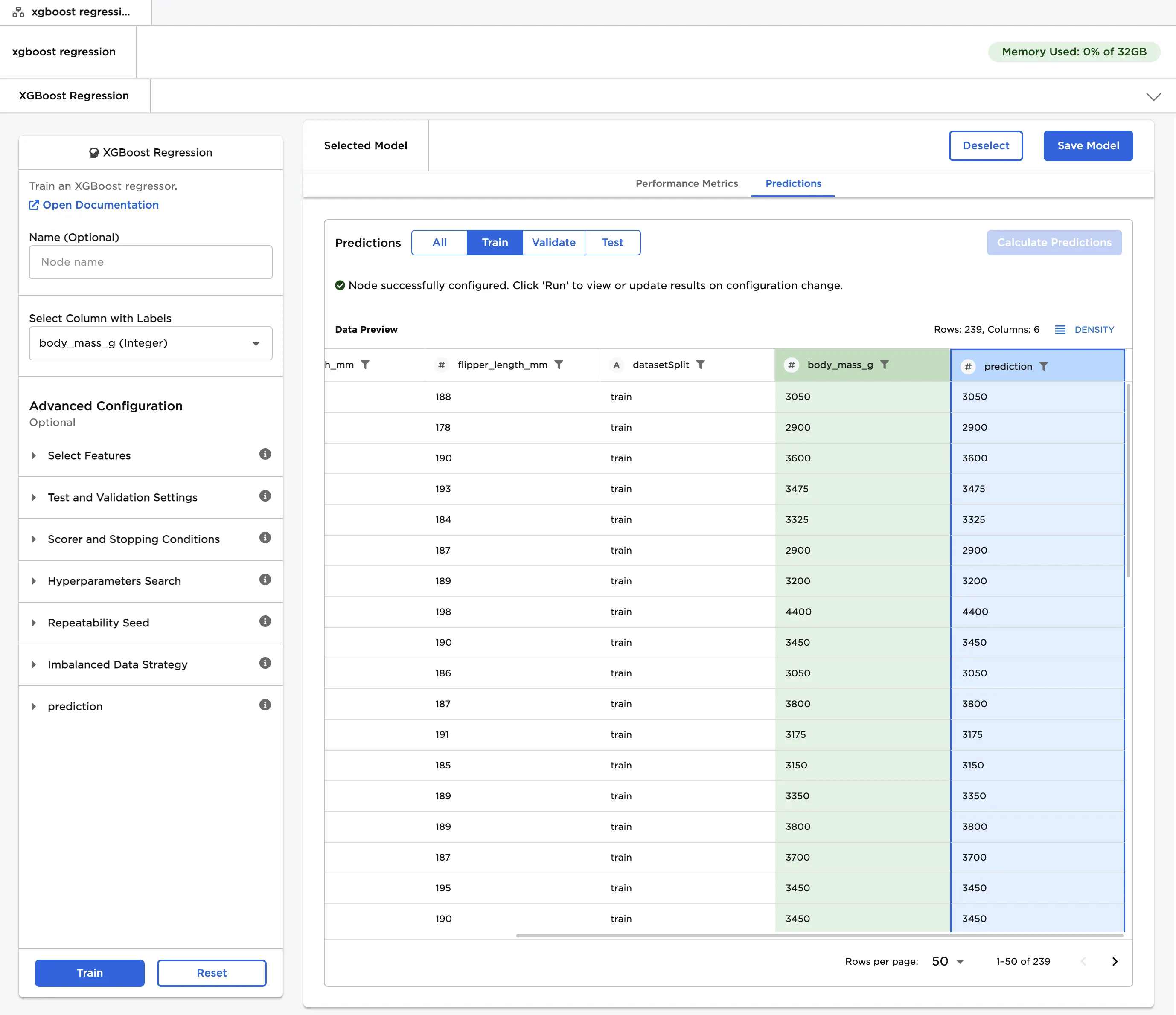
Figure 1: Example output
Examples
The dataframe shown in Figure 2 contains identifying characteristics of over 300 penguins. This data is used to train a model that can predict a penguin's body mass given its bill length, bill depth, and flipper length. This is a regression problem because you are trying to predict a continuous, numeric value.
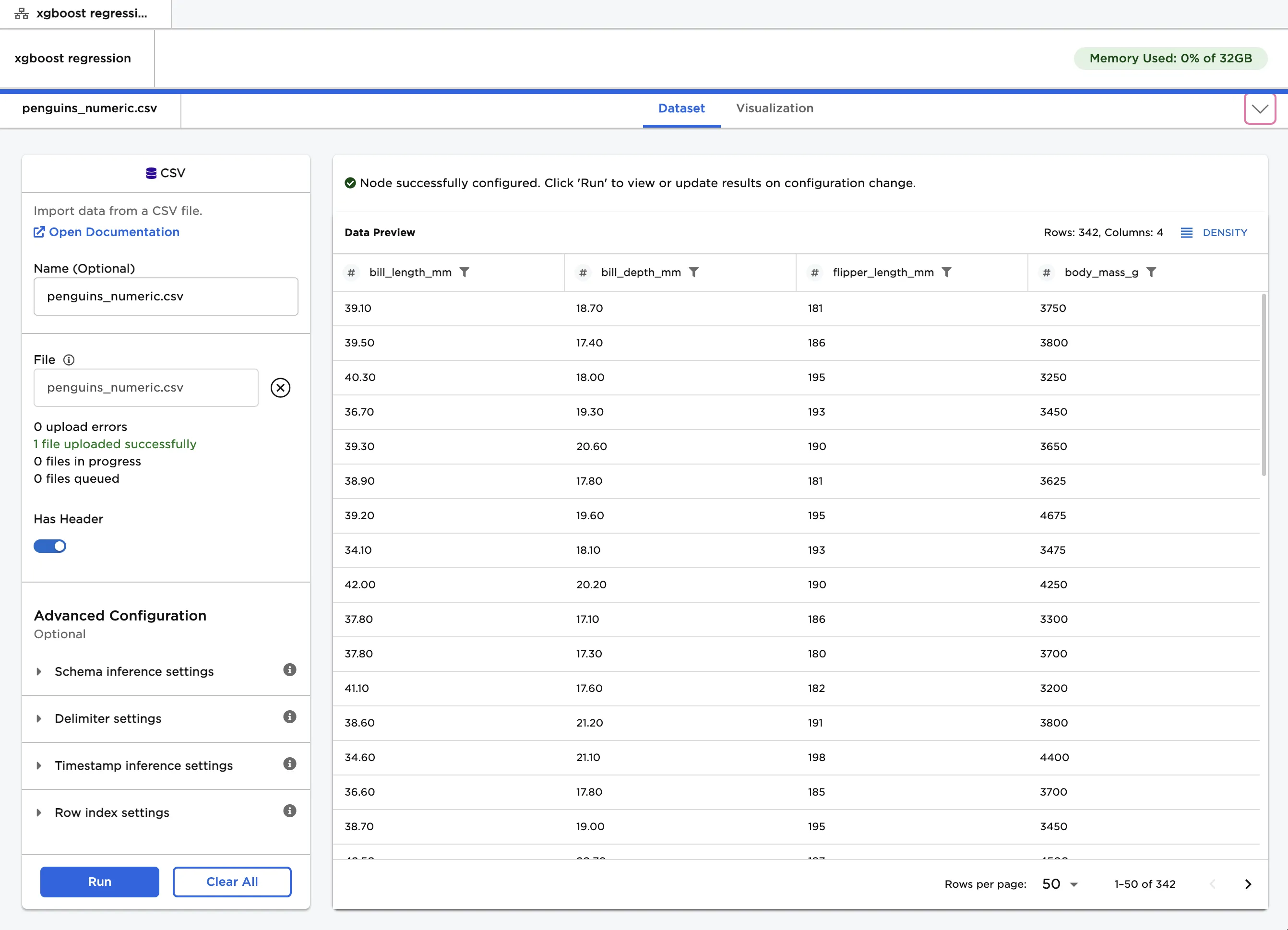
Figure 2: Example input data
- Connect an XGBoost Regression node to an existing node.
- Select body_mass_g (Integer) for the Select Column with Labels field. The model should be able to predict the values in this column after training.
- Select Train to train models with the default settings.
Notice that Visual Notebooks trains multiple models, each with different hyperparameter configurations. All trained models are displayed on a leaderboard and ranked by performance.
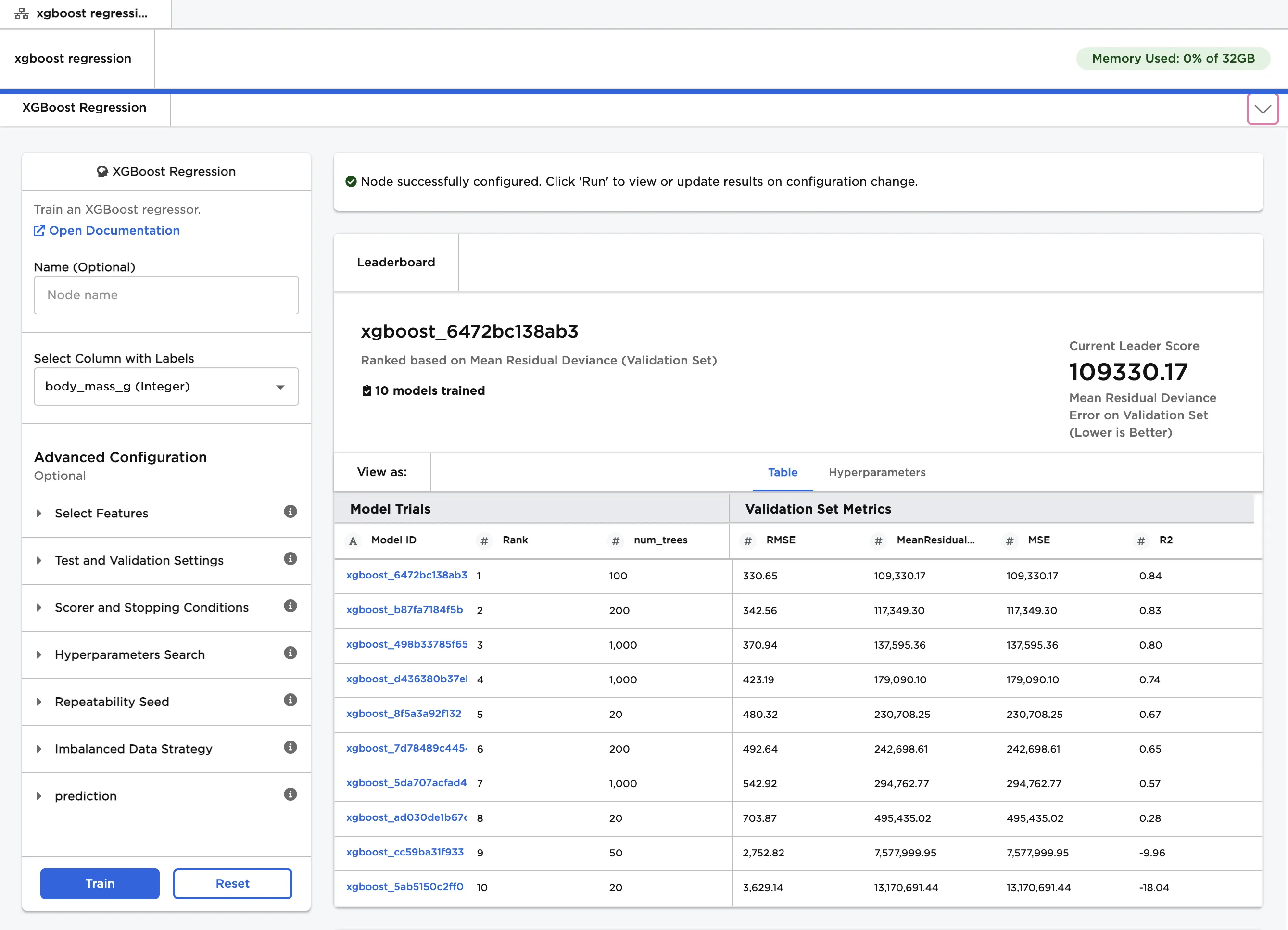
Figure 3: Model leaderboard
- Select a model, then scroll down to view information about the model and a bar chart with the importance of each feature.
- Select Calculate Additional Details to view additional test metrics and a scalar regression chart. The button appears dimmed after it has been selected. For more information about test metrics, see the Visual Notebooks User Guide.
The scalar regression chart shows the model's predictions as a gray line. The actual values are displayed as blue dots. Although the model in Figure 4 does not accurately predict all values, it successfully captures the general trend of the data.
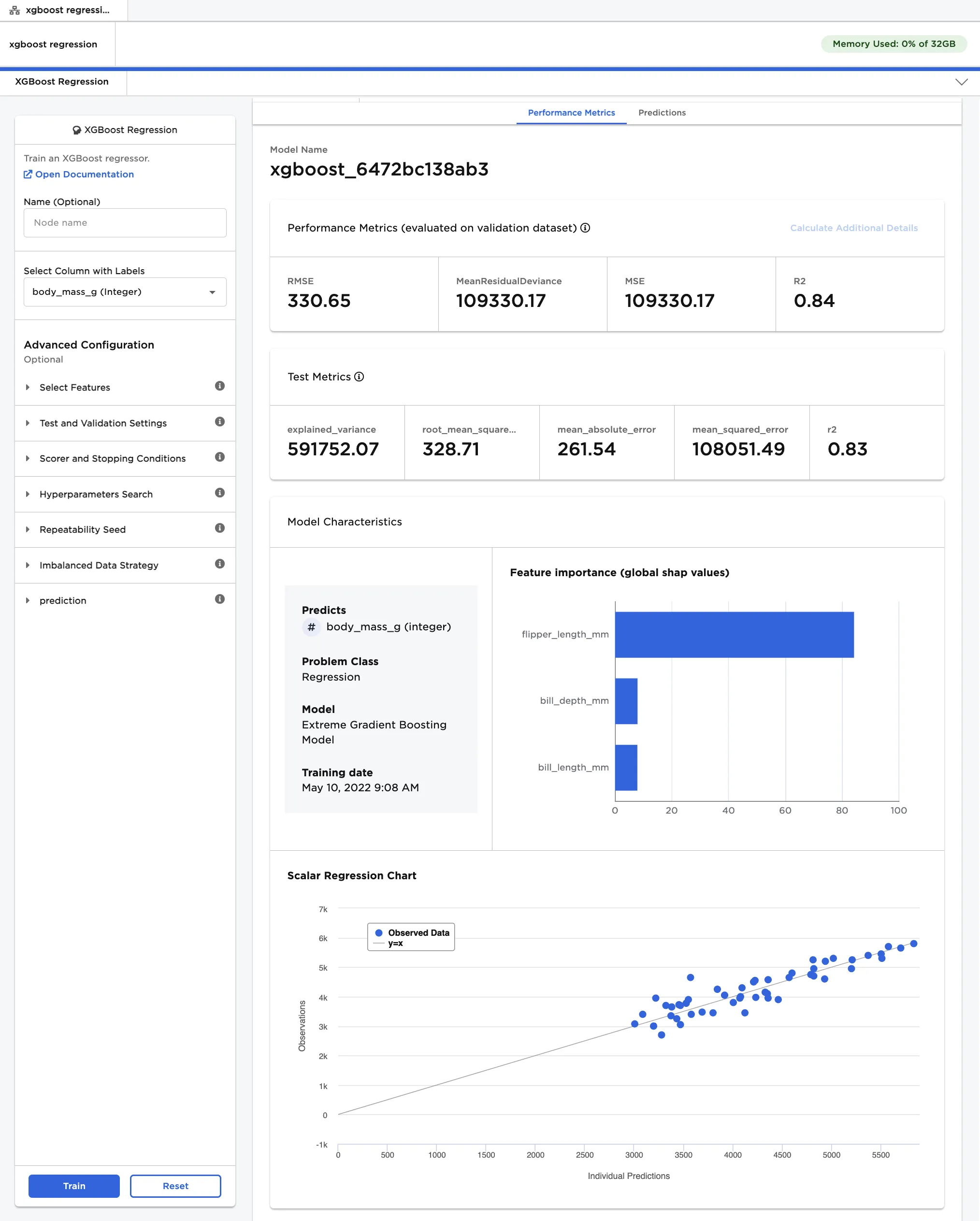
Figure 4: Model details
- After a model is selected, navigate to the Predictions tab.
- Select Calculate Predictions to view the selected model's predictions on the training data. The button appears dimmed after it has been selected.
If the leading model doesn't perform as well as you'd like it to, try altering the advanced configuration options and training new models.
Note that if your model correctly predicts all values, it might be overfit. In other words, the model may be too closely aligned to the training data to make accurate predictions on unseen data. Try altering the hyperparameters or using a different AutoML node.
Figure 5: The selected model's predictions