Understand Normalization
Normalization is a feature that transforms raw time series data into a more structured time series, and stores it in a C3 AI data store for faster access and analysis.
When ingested, often IoT sensor data contain duplicates, overlapping values, or otherwise inconsistent formatted data from disparate sources. The Normalization Engine converts these raw time series data points into structured, normalized time series data, which can be used to draw meaningful insights and analysis through exploration, charting, and machine learning algorithms.
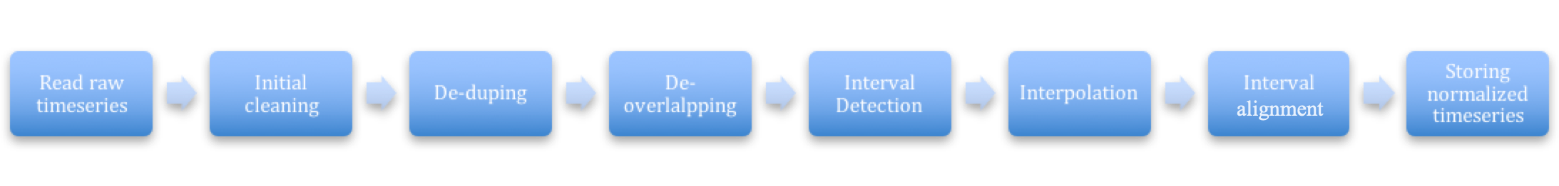
The data are structured and normalized through a preprocessing pipeline that includes data cleaning, unit conversion, de-duplication, de-overlapping, interpolation, and interval alignment. Normalization preprocessing resolves for gaps, duplicates, overlaps, and other data issues, so that any application developer, data scientist, or analyst can start with clean, preprocessed data for their exploration, analysis, and applications.
Normalization data categories and Types
A time series is a sequence of data points over a period of time. The platform categorizes these into two main categories:
- Interval: Time series where each data point has an explicit start and end timestamp, indicating the value for an interval. For example, an energy bill provides a specific duration, or dedicated period of time with an explicit start and end timestamp. See IntervalDataPoint.
- Point: Time series where each data point has only a timestamp, indicating when the event happened. For example, a temperature reading is taken at a particular instant in time. See the TimedDataPoint Type which mixins this Type to store raw time series data points which happen at a point in time.
An example DataPoint Type derived from a raw IoT sensor reading could be as follows.
type DataPoint {
  /**
   * ID of the sensor sending the data point
   */
  sensorId: !string

  /**
   * Start date for this sensor reading
   */
  start:    !datetime

  /**
   * End date for this sensor reading. The end is populated only if the time series is Interval
   */
  end:      datetime

  /**
   * Value recorded by the sensor for this time period
   * The data type of the time series field can be (float, double, decimal, integer, Dimension, ExactDimension)
   */
  value:    !double

  /**
   * Unit of the value recorded For example, kilowatt_hour
   */
  unit:     string
}
Each series of values are associated with two Types in the Type system.
Actual data points: This data structure is a Type that contains the actual reads from the sensor and is similar to the the structure noted in the above example. To qualify as a data point, the Type should mixin either IntervalDataPoint or TimedDataPoint.
Meta about the data points (series header): This Type contains metadata about the actual time series data points and might include details about how the data points should be normalized. To qualify as a time series header, the Type should mixin either IntervalDataHeader or TimedDataHeader.
NOTE: For the normalization process to work, the above Types must be created and mapped correctly. That is, there must be a one-to-one mapping between a IntervalDataPoint Type and IntervalDataHeader Type, or a one-to-one mapping between a TimedDataPoint Type and TimedDataHeader Type, depending on the category of time series data in the data set.
Normalization process
The set of raw time series data points goes through the following steps to be normalized.
See Time Series Data Treatments for more information on aggregation operations that can be used for normalizing your data.
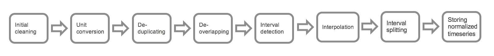
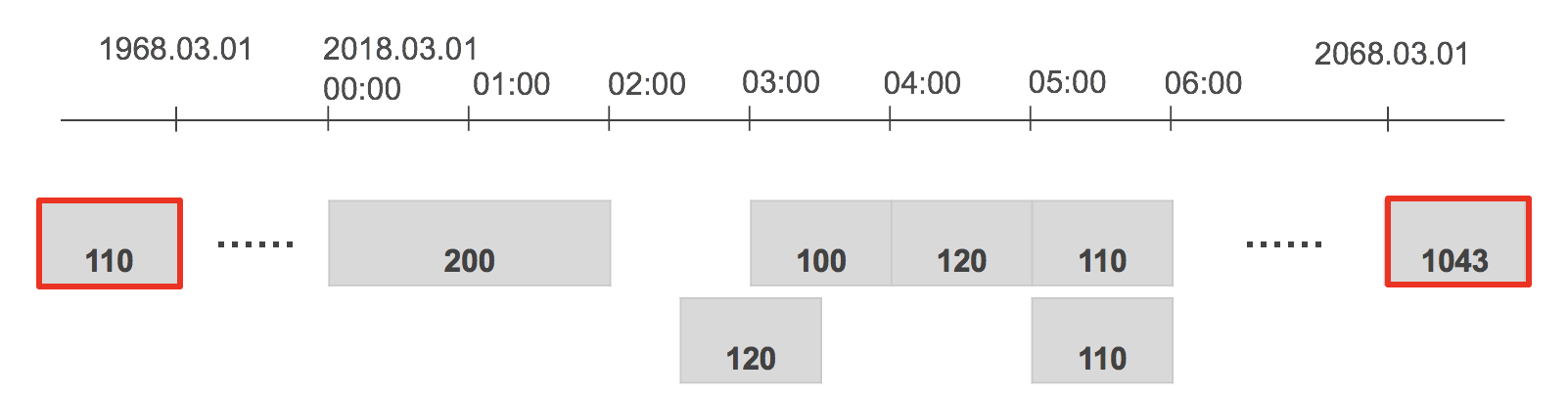
1. Initial cleaning
This step includes cleaning the data points and rejecting bad data points.
The following considerations are part of this stage in the process:
- Sets timezone of start and end (if applicable) to the normalization timezone. For example, if this is a legacy data point (when normalization was using noon UTC for start of day instead of 00:00 hours), this process corrects the start and end accordingly.
- Rejects data points that have no value.
- Rejects invalid data points. For example, this process rejects data points that are:
- Greater than 50 years from start and end date.
- More than 50 years from the current date either as start or end date.
- Removes timezone information from the raw data and stores it for timezone related queries.
2. Unit conversion
This step is responsible for ensuring that the entire time series has a homogeneous unit. See the Unit Type for a library of units offered for use with calculations.
The following considerations are part of the unit conversion stage in the time series normalization process:
- Identify what the normalization unit for the time series attribute is from the annotation/parent field, using the following parameters, which are listed in order of importance:
- Annotation @ts(unitPath="path.to.unit") - This annotation exists on the time series field and gets the maximum preference. The unit path indicates the value of the unit. This path can point to a string or a unit object.
- Annotation @numerical(requiredUnit=UnitObject) - Legacy annotation numerical on the time series field can directly specify the unit object. This path can point to a string or a unit object.
- Annotation @numerical(unitPath="path.to.unit") - Legacy annotation numerical on the time series field can specify path to unit. This path can point to a string or a unit object.
- Time series field is ExactDimension or Dimension - If one of these is on the time series field, the value of the
unitfield is picked from the first non-null data point in the raw time series and all the other points are converted to that. - Time series header mixes TimeseriesInfo - If the time series header mixes
TimeseriesInfo, the value of the unit is determined by theunitfield on theTimeseriesInfoobject.
- If an error occurs while figuring out what the unit for the time series is, the exception is caught and logged as a warning and normalization continues. If the unit was determined accurately, normalization stores this unit as a part of the normalized time series for later use. (See NormalizedTimeseries for more information.)
- While specifying
unitPath, you can either chose to includeparent, or directly specify theunitPathon the parent withoutparent.
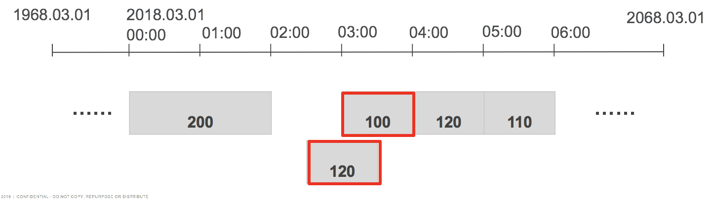
3. Handling duplicates
This step figures out if a data point is a duplicate of the other. A data point is considered a duplicate if start, end, unit, value(close enough), isEstimated, dataVersion are the same on the data point Type that mixes in either IntervalDataPoint or TimedDataPoint.
There are two types of duplicate handling for each time series that can be set on the series header:
- IGNORE (default): This means if the two consecutive points are duplicates of each other, the second point is ignored.
- KEEP: This means if the two consecutive points are duplicates of each other, both data points continue through normalization processing.
NOTE: Duplicate handling can be overridden by setting the duplicateHandling field on your series header.
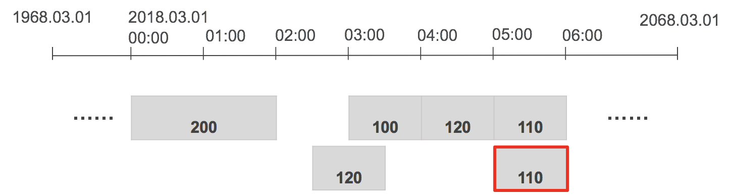
4. Handling overlapping data points
This step in the normalization pipeline makes sure that there are no overlapping data points in the subsequent steps of the pipeline. See also overlapHandling in TSDecl.
Overlapping points can be handled in the following ways:
- AVG (default): De-overlapped data point is an average of all overlapping data points.
- SUM: De-overlapped data point is the sum of all overlapping data points.
- MIN: De-overlapped data point is the minimum of all overlapping data points.
- MAX: De-overlapped data point is the maximum of all overlapping data points.
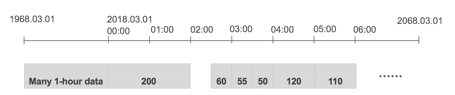
5. Interval detection
This step determines the natural interval of the raw time series data. The algorithm looks at the first 100 raw data points and deduces the interval of the raw data.
Specifying the interval skips this step. You can enforce normalizing the time series at a particular interval by specifying IntervalDataHeader#interval or TimedDataHeader#interval.
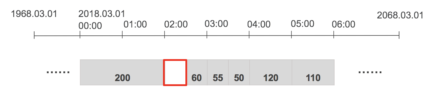
6. Interpolation
This step is responsible for interpolating values between two interval data points if the end of the first point is not the start of the next point.
Interpolation can be handled in one of the following ways:
- ZERO INTERPOLATION (default): Puts 0 values for gaps.
- LINEAR INTERPOLATION: Draws a line between the two points and then fills the intermediate value with the midpoint of the line.
Linear interpolation calculates the intensity of the gap by drawing a straight line from the midpoint of the first raw data point to the midpoint of the second raw data point for the intensity. The value of the gap is calculated by multiplying the intensity of gap by the width of the gap. See the following equation for reference.
$$
(v - v1) / (t - t1) = (v2 - v1) / (t2 - t1)
v = (v2 - v1) / (t2 - t1) \times (t - t1) + v1;
$$NOTE: If the point spans multiple grains, then the midpoint of the line is divided equally into separate grains instead of linearly increasing values. See also GrainDetector and GrainSplitter.
7. Interval alignment
The interval aligner is responsible for aligning the interval data points to calendar-aligned dates for that interval. For example, if a monthly bill spans from Jan 15th to Feb 15th, the interval aligner splits this point into two pieces, one for Jan 15th to Feb 1 (exclusively) and other from Feb 1 to Feb 15, then appropriately assigns the values to the corresponding months based on the treatment specified.
The aggregation or disaggregation of the data is performed based on which is specified on the IntervalDataHeader or TimedDataHeader.
Pre-aggregation
Pre-aggregation is an optimization step in the normalization process. It involves summarizing data at common intervals and storing these summaries to speed up data retrieval. This reduces the need for real-time computation when the data is queried.
Key concepts
Normalization Interval: This is the interval at which raw time series data is normalized and stored. Examples include minute, hour, day, and month.
Pre-aggregated Intervals: These are common intervals for which the system pre-computes and stores summary data. This helps in quick retrieval and reduces computational load during queries.
How pre-aggregation works
When raw data is normalized, it’s typically done at a specific interval (for instance, minute, hour, day, month). For each normalization interval, the system computes pre-aggregated data at one or more broader intervals. This is done for efficiency and faster access. The table below shows the mapping:
| Normalization Interval | Pre-aggregated Intervals |
|---|---|
| MINUTE | QUARTER_HOUR, HOUR, DAY, MONTH |
| QUARTER_HOUR | HOUR, DAY, MONTH |
| HOUR | DAY, MONTH |
| DAY | MONTH |
Raw data is first normalized at the specified interval. During normalization, the system also calculates summary data for pre-aggregated intervals. For example, if the data is normalized at the minute level, the system can also compute hourly, daily, and monthly summaries. These summaries are stored in a pre-aggregated format. This means if a user queries the data at these common intervals, the system can return the pre-aggregated results without recalculating them.
Benefits of Pre-aggregation
- Reduced Computation: By storing pre-aggregated data, the system avoids recalculating aggregates every time a query is made, significantly speeding up data retrieval.
- Improved Performance: Pre-aggregation helps in handling large volumes of data efficiently by reducing the input/output operations required for real-time calculations.
- Optimized Storage: Despite additional storage requirements for pre-aggregated data, the overall performance gain justifies the trade-off, making data access quicker and more efficient.
Handling queries with pre-aggregated intervals
When a query is made for an interval that matches one of the pre-aggregated intervals, the system directly retrieves the pre-aggregated data. This ensures fast query responses as no further computation is required. However, if a query is made for an interval that is not pre-aggregated, the system performs in-memory aggregation/disaggregation from the nearest pre-aggregated interval.
For example, if you need a weekly average and it’s not pre-aggregated, the system might compute it from daily averages.
Example of pre-aggregation in action
Imagine you have temperature sensor data recorded every minute. The normalization process normalizes this data at the minute interval. However, for frequent queries at broader intervals, such as hourly, daily, or monthly average temperatures, pre-aggregated data is computed and stored.
- Minute-level Data: The raw temperature readings are normalized and stored every minute.
- Hourly Aggregation: The system calculates and stores the average temperature for each hour.
- Daily Aggregation: It also calculates and stores the daily average temperature.
- Monthly Aggregation: Finally, it computes and stores the monthly average temperature.
When a user queries the average temperature for a particular day, the system can directly retrieve the pre-aggregated daily data instead of recalculating it from minute-level readings. This results in much faster query responses.
Interactions between pre-aggregation and treatments
Treatments applied to the time series data during normalization also impact how pre-aggregation works. Treatments define how raw data points are transformed during normalization. For example, an average (AVG) treatment can calculate the mean value of data points within each interval.
When pre-aggregated data is used, the system ensures that the treatment rules are consistently applied. For instance, if the data is treated with AVG, the pre-aggregated values at higher intervals (for instance, hourly) are averages of the lower interval data (minute-level data).
Customizing pre-aggregation
Users can configure pre-aggregation to align with their specific use cases by:
- Choosing Intervals for Pre-aggregation: Selecting appropriate intervals for pre-aggregation depends on the most common query patterns and the nature of the data.
- Balancing Storage and Performance: Pre-aggregated data increases storage requirements but significantly boosts
performance. The balance between these factors is crucial for system efficiency.
Implementation considerations
- Setting Pre-aggregation Intervals: You can specify which intervals to pre-aggregate by configuring the time series header. For instance, you might pre-aggregate minute-level data into hourly and daily intervals.
- Handling Changes in Data: When new data arrives or changes are made, the pre-aggregated data must be updated to reflect these changes accurately.
Troubleshooting Common Issues with Pre-aggregation
Normalized values not as expected
If you notice discrepancies in normalized values, check the following:
- Treatment Application: Ensure the correct treatment is applied to the series header. This determines how the data is normalized.
- Pre-aggregation Logic: Verify the intervals and the logic used for pre-aggregation. Discrepancies can arise if the pre-aggregated values do not align with the expected grain.
Pre-aggregation vs. TsDecl metrics
Normalized metrics using pre-aggregation and TsDecl metrics behave differently by design:
- Normalized Metrics: Pre-compute at three levels of aggregation and then aggregate/dis-aggregate from those.
- TsDecl Metrics: Always aggregate directly from the raw data, without intermediate steps.
If you encounter issues with pre-aggregated metrics, consider using TsDecl metrics for direct raw data aggregation, which can provide more precise results in some scenarios.
Pre-aggregation is a strategic step in the normalization process that optimizes data retrieval by storing summarized data at common intervals. This ensures quick and efficient access to time series data for analysis and reporting, enhancing the overall performance of the C3 Agentic AI Platform.
8. Storage
The last stage of the normalization is process is storing the normalized values in the time series storage. After the series has been normalized using the steps above, it is then persisted in a compact, columnar format in a time series database in the C3 Agentic AI Platform for fast retrieval on reads. The structure of the normalized time series is represented by the NormalizedTimeseries Type.
New change and incremental normalization
In cases in which new time series data points are constantly loaded into the C3 Agentic AI Platform and the normalization process should not be engaged each time, the Incremental Normalization process is employed. This process only normalizes the recent, raw time series data rather than re-normalizing the entire time series data set each time.
By default, Incremental Normalization is disabled to ensure the additional data load doesn't negatively impact the system while the data load is in progress.
Configure normalization to modify how data is normalized on arrival or when changed by using the following example code snippet.
NormalizationConfig.make().setConfig("mode", "YOUR_NORMALIZATION_MODE");When new data arrives or changes are made to the data points, the normalization engine marks the NormalizedTimeseries instance (if it exists) associated with series header as invalid. The next time normalized data are accessed for the series, the normalization process attempts to normalize the series before serving the request.
However, you can configure normalization to process immediately when data are changed or when new data arrives to ensure the request is not delayed.
To configure the normalization, use one of the following values:
ALL: Normalizes the series with new data arrival or data change, irrespective of whether the series was previously normalized or not. This causes an entry to be put in the NormalizationQueue for every series header for which data has changed or new data arrived with the time range information of the duration of the data points.
If the normalized data is requested before the entry in the NormalizationQueue is processed, then the current data stored in the NormalizedTimeseries object is returned as is without attempting to re-normalize since an entry is already there in the NormalizationQueue. This state will be consistent, eventually. Therefore, there is no delay in serving the normalized values in this mode.
RECENT: Normalizes the series with new data arrival or data change ONLY if the series was previously normalized. This enables you to only normalize data that is being accessed by the application and not everything that is loaded in the platform. This helps in saving storage and time by only normalizing series that are actively accessed. This causes an entry to be added in the NormalizationQueue for the series header for which data has changed or new data has arrived with the time range information of the duration of the data points. The series is normalized incrementally.
If the normalized data is requested before the entry in the NormalizationQueue is processed, then the data is normalized on that read operation and there is a delay in serving the normalized data. However, if the entry has already been processed, then there is no delay in serving the normalized values.
ONDEMAND (default): Invalidate the series to perform INCREMENTAL normalization when new data has arrived since the last request of normalized data. No entry is put in the NormalizationQueue in this mode and there is a delay in the response. Subsequent requests of normalized data won't experience response delay (provided new data has not arrived).
AFTERQUERY: Normalizes the series with new data arrival or data change, ONLY if the series was previously normalized. This enables you to only normalize data that is being accessed by the application and not everything that is loaded in the platform (similar to RECENT). This causes an entry to be put in the NormalizationQueue for the series header for which data changed or new data has with the time range information of the duration of the data points. The series is normalized incrementally.
If the normalized data is requested before the entry in the NormalizationQueue is processed, then the current data stored in the NormalizedTimeseries object is returned as is without attempting to re-normalize and an entry is added in the NormalizedTimeseries to normalized the series with full normalization. However, if the entry is processed already, then there is no delay in serving the normalized values unless the series has never been normalized.
See NormalizationMode for details.
Estimated or actual value in time series data point
Occasionally, it is necessary to specify whether the data value isEstimated or the actual value. For example, a utility company sends you an estimated bill for your usage and then later sends you the actual bill value for your usage. Both of these data points are loaded in data point Type (by setting the TimedDataPointFields#isEstimated on each data point). The normalization process handles these data points using the following parameters:
- If an actual value exists, use the actual value for normalization.
- If actual and estimated readings exist for the same interval, normalization should use the actual value (estimated values are ignored).
- If only an estimated value exists in an interval, the estimated value is used in normalization and identified as an estimate.
TimeZone handling
By default, the series is normalized in the TimeZone of the source of the data and stored in the time series database. When a series is evaluated using Persistable#tsEval or MetricEvaluatable#evalMetric, the default time zone is TimeZone#NONE; that is to say, the data are returned based on how they were stored in the database without applying any time zone transformations.
Consider the following query as an example.
var ts = UtilityBillSeries.tsEval({
  projection:"sum(normalized.data.usage)",
  start:"2015-01-01T00:00:00",
  end:"2015-01-01T03:00:00",
  grain:"HOUR",
  filter:"id == 'customer-1'",
  timeZone:"NONE"}).data();
When a query is made to retrieve these data with the default time zone, the normalized values are returned as shown below.
Actual Values:
                        10                             20                            30
          |------------------------------|------------------------------|------------------------------|
  Jan1 00:00-08:00              Jan 1 01:00-08:00             Jan 1 02:00-08:00              Jan 1 03:00-08:00

Normalized Values:
                        10                             20                            30
          |------------------------------|------------------------------|------------------------------|
  Jan1 00:00-08:00              Jan 1 01:00-08:00             Jan 1 02:00-08:00              Jan 1 03:00-08:00
However, there are disparate sources of data in which the time zone in one source is offset with +04:00 and the other with -08:00 and they must be transformed to the same time zone, you can normalize the time zone data explicitly. See TimeZone and Understanding Time Zone Data for more information.
Hot/cold normalized storage
Normalized data occupy a significant amount of space in the Cassandra cluster. If latency of retrieving data from cold store is not a concern or if the query patterns seldom touches old data, then it is a better to leverage the hot/cold storage for storing normalized data. To enable hot/cold storage, do one of the following:
Set the hot/cold storage per data point type. This applies to ALL headers on the time series Type.
JavaScriptNormalizationConfig.make({ partitionStrategy: { "MyDataPointType": { "maxHotBucketDate" : "now() - period(3, 'MONTH')" } } });Set hot/cold per time series header. This only applies to the headers where this configuration is specified. This also takes precedence in case both configurations are set.
JavaScriptMyTsHeaderType.make({ normalizationPartitionStrategy: { "maxHotBucketDate" : "now() - period(3, 'MONTH')" } }).upsert();
See NormalizationPartitionStrategy and NormalizedTimeseriesHotColdMigrator for more information.
Cold storage data refresh
By default, CronJob is triggered every month to move the data from hot store to the cold store. Alter the cron job and change the cadence as desired for your application. The cron job id to search for is: "trigger-normalizedtimeseries-hotcold".
If normalization touches data in the cold store while normalizing, then the data is directly merged with an existing file in the cold store or a new one is created if it does not already exist. No manual intervention is required for this to be enabled.
See CronConfig and CronSchedule.
Custom normalization
Customize the normalization processes as desired by following the example steps below. See NormalizationConfig and Normalizer.
Step 1: Create a Type that mixes Normalizer
/**
 * Dumb normalizer where it returns the same value as in the data points
 */
type IdentityNormalizer mixes Normalizer {

  /**
   * Function that needs to be overriden
   */
  normalize: function(objs: stream<TSDataPoint>, spec: TSNormalizationSpec): [Timeseries] js-server
}Step 2: Implement the normalization logic
The normalization logic can be more complex then shown below. For the purpose of this example, we are returning the same data points as those in the raw data.
/**
 * This is a custom normalizer. This function should look at data points and then create Timeseries per month
 */
function normalize(objs, spec) {
  var results = [];
  var i = 0;
  while (objs.hasNext()) {
    var current = objs.next();
    if (current.value == null)
      continue;
    var ts = Timeseries.fromValue(TimeInfo.make({
      start : current.start,
      end : current.end,
      interval : "MONTH" }), current.value, current.unit != null ? current.unit : null);
    results[i++] = ts;
  }
  return results;
}
There are several helper functions from the original normalizer to help you normalize the data. See GrainDetector#detectGrain, GrainSplitter#align, and Unit#getConversionFactor for details. You can also view more complex custom normalizer implementation, which is already in the C3 Agentic AI Platform by running the following code snippet:
RegisterNormalizer.sourceCode("JavaScript")Normalization tutorial
Use the following normalization tutorial to walk through your use case.
Step 1: Identify the nature of your data
The first step is to identify the nature of the data. Follow these steps to chose the right Types for your application
- Identify if your data is Interval or Point as discussed at the beginning of this document.
- If Interval, then ensure your data point Type mixes IntervalDataPoint (with end) and series header mixes IntervalDataHeader.
- If Point, then ensure your data point Type mixes TimedDataPoint (no end) and series header mixes TimedDataHeader.
- Identify if your data points are high frequency (finer than 5 minute interval) data points and need to store raw data points in file based, cheaper storage.
- If it does, then ensure to use hot/cold storage to store data in cold store.
Step 2: Create types
In the following examples, the default storage option is used. Define the Types as follows based on whether there is interval data or point data.
Header type:
 entity type UtilityBillSeries mixes IntervalDataHeader<UtilityBill> schema name 'UBS' {
   /**
      * Unit of currency
    */
   currencyUnit : !string
 }
DataPoint type:
  @db(datastore='kv')
  entity type UtilityBill mixes TimeseriesDataPoint<UtilityBillSeries> schema name 'structure_UtilityBill' {
    /**
     * Time series field to track actual usagae
     */
    @ts(treatment='integral', unitPath="parent.currencyUnit")
    usage : !double
}Step 3: Set techniques to apply during normalization like treatment and unit
After you have defined the Types, consider whether the following should be specified:
Treatment: How you want the values to be normalized. See Time Series Data Treatments to find out the various treatments are applied during the normalization process and can be set by providing treatment on the Ann.Ts annotation on the time series field.
Unit: Determine from where the unit for normalization should be determined from. It is not necessary to select the unit for the normalization process to run.
Time series annotations
Specify annotations on a time series field to indicate how to normalize a time series. See Ann.Ts and Ann.Normalization for details.
Step 4: Load data
After the Types have been created, you are ready to load data into these Types.
End-to-end normalization tutorial
This tutorial is a step-by-step guide to normalize an interval time series (that is, a time series that has both start and end values in their data points). In this example, the use case is creating time series for storing daily utility bills in the C3 Agentic AI Platform.
Step 1. Create a time series header Type for metadata
Create a time series header type that holds metadata about how this time series must be normalized. All the fields that instruct the normalization engine to apply specific rules comes from the IntervalDataHeader Type.
In the following example, the header type UtilityBillSeries mixes in IntervalDataHeader. This header type needs to provide the data point Type that it is connected to it, so that the normalization engine knows that the actual time series data points should be retrieved from the this data point Type.
Create a file with filename: UtilityBillSeries.c3typ
entity type UtilityBillSeries mixes IntervalDataHeader<UtilityBill> schema name 'UBS' {
  /**
   * Unit of currency
   */
  currencyUnit : !string
}Step 2. Define the data point Type holding the time series data points
Define the data point Type that holds the actual time series data points. This Type also must be linked to the time series header to which it is associated.
Let the data point type be called UtilityBill (referenced above from the series header) that mixes in IntervalDataPoint.
Create a file with filename : UtilityBill.c3typ
@db(datastore='kv')
entity type UtilityBill mixes IntervalDataPoint<UtilityBillSeries> schema name 'structure_UtilityBill' {
  /**
   * Time series field to track actual usagae
   */
  @ts(treatment='integral', unitPath="parent.currencyUnit")
  usage : !double
}
This example Type above indicates that the data points are going to be stored in Cassandra and the time series field is usage. Apply AggOp#INTEGRAL to it and the unit for this data can be obtained from the header field currencyUnit.
Step 3. Create dummy data to continue example
For this example, create dummy data for the header and the data point Types using the functions provided below.
// One time series belonging to one customer who has daily bills between 5 and 10 dollars
function createMeasurement () {
  var parentId = "customer-1";
  UtilityBillSeries.upsert(UtilityBillSeries.make({id: parentId, currencyUnit: {id:"dollars"}}));
  var no = 365 * 2;
  measurements = [];
  var startDate = Date.deserialize("2015-01-01T00:00:00");
  for (var i = 0; i < no; i++) {
    var dpStart  = new Date(startDate.getTime() + (i * 24 * 60 * 60 * 1000));
    var dpEnd = new Date(dpStart.getTime() + (24 * 60 * 60 * 1000));
    measurements.push(UtilityBill.make({start: dpStart, end: dpEnd, usage: (Math.floor(Math.random() * (10 - 5 + 1)) + 5), parent: {id : parentId}}));
  }

  if (measurements.length > 0) {
    UtilityBill.upsertBatch(measurements);
  }
  return parentId;
}

createMeasurement();Step 4. Normalize the time series manually
After raw data has been created, normalize the time series manually using the following code snippet.
UtilityBillSeries.normalizeTimeseries(UtilityBillSeries.make({id:"customer-1"}))The data is automatically normalized on read if it has not been previously normalized. For this example, assume that this time series is read directly instead of manually normalizing; the normalized values would still result.
var ts = UtilityBillSeries.tsEval({
  projection:"sum(normalized.data.usage)",
  start:"2015-01-01",
  end:"2017-01-01",
  grain:"DAY",
  filter:"id == 'customer-1'"
});
c3Viz(ts);Troubleshooting and debugging
Check if a series has been normalized
There are a few steps that you can take to verify whether a series has been normalized correctly or not.
Find the key for normalized time series object using the API IntervalDataHeader#normalizedTimeseriesKey. (See TimedDataFields)
After you have the key, you can retrieve the normalized time series object using the API NormalizedTimeseriesPersister#getId.
- Inspect this object to see if there are any errors in the error field on the NormalizedTimeseriesState object. If there are, correct the errors and re-normalize the time series.
- Also, inspect this object to ensure that the field NormalizedTimeseries#valid is set to true, which means that the series is normalized and ready for consumption.
For example,
JavaScriptNormalizedTimeseriesPersister.getId(PhysicalMeasurementSeries.normalizedTimeseriesKey('YOUR_MS_ID', 'TS_FIELD_NAME'));To verify whether a series has been normalized or not, check the earliest and latest field on the time series header.
Total time range of normalized data
Inspect the earliest and latest field on the series header to find the total range of normalized data.
Querying normalized data
Query normalized data using tsEval on the time series header.
For example,
PhysicalMeasurementSeries.tsEval({
  projection:"sum(normalized.data.quantity)",
  start:"2010-01-01",
  end:"2011-01-01",
  interval: "MONTH",
  filter:"id == 'YOUR_MS_ID'"
});Troubleshooting common issues
Normalized values are not expected
Check the TSDecl#treatment Type is being applied on the series header, which determines how the series is normalized.
Even after creating Types, the data are not getting normalized
One of the common mistakes is to forget marking the time series field with the @ts annotation.
For example, notice the @ts annotation on the usage field in the following example. This is required for trigger normalization.
@db(datastore='kv')
entity type UtilityBill mixes IntervalDataPoint<UtilityBillSeries> schema name 'structure_UtilityBill' {
  /**
   * Time series field to track actual usagae
   */
  @ts(treatment='integral', unitPath="parent.currencyUnit")
  usage : !double
}fetchNormalizedData failed: Could not find definition of unit in database
This indicates that the unit was present in the database when the series was normalized and you need to create a definition of the unit on the Unit Type and re-normalize the series.
Miscellaneous common errors
See these links for more information:
Limits
Total number of lock attempts
Before normalization begins, a DbLock is acquired on the series header, which restricts the same series from being concurrently normalized within the cluster. Currently, the normalization engine attempts to acquire a lock 10 times with a delay of 100 ms in between the two checks after which, it fails with Could not acquire lock exception.
These errors are re-tryable. You can simply retry the normalization by recovering failed jobs on the queue, or by simply requerying. If there is high content, then you can raise the number of retries using the following code snippet.
NormalizationConfig.make().setConfigValue("maxLockAttempts", 100); // retries 100 times instead of 10 (default)Data types
The value type that can be used as the time series field are limited to: float, double, decimal, integer, boolean, Dimension, ExactDimension.
Key points to consider in disaggregating data
Consistency: The behavior differs based on whether the data is pre-normalized or normalized on the fly. This can lead to discrepancies, especially across different time zones.
Time zone impact: When a time zone that matches the TimedDataHeader's time zone is requested, the pre-normalized data is used, and disaggregation occurs. However, when a different time zone is requested, normalization happens on the fly, and data is not disaggregated.
Performance: Normalizing data on the fly may cause a performance hit, and the lack of disaggregation leads to data being returned at specific timestamps rather than evenly across the requested interval.
The Metric Engine does not consistently disaggregate data to finer intervals when generating timeseries on the fly. This inconsistency arises depending on whether the data is pre-normalized or normalized on the fly:
Pre-normalized data:
When data is pre-normalized to a certain interval, for instance,
DAY, and a finer interval such asHOURis requested, the Metric Engine disaggregates the data to the requested interval. This means the daily data is evenly split into hourly data points.- Example: Daily data disaggregated into hourly data points.
On the fly normalization:
When the timeseries is generated on the fly, the Metric Engine does not disaggregate the data to finer intervals. Instead, it assigns the full value to the single interval that contains the raw timestamp of the data.
For example, if daily data is requested as hourly, the entire day's value is assigned to a specific hour rather than being spread across all hours.
- Example: Daily data assigned to a specific hour without disaggregation.
API reference
A time series in the C3 Agentic AI Platform is automatically normalized behind the scenes:
- On read, if it hasn't previously been normalized or has been marked invalid due to new data arrival.
- Incrementally, if the series has been marked to be normalized using the environment.
Automatically normalizing time series data might affect performance while running high throughput analytics. Use the following APIs to normalize time series manually to reduce the impact.
Synchronous
To normalize time series and persist the values to the NormalizedTimeseries Type use TimedDataFields#normalizeTimeseries.
For example,
JavaScriptPhysicalMeasurementSeries.normalizeTimeseries(PhysicalMeasurementSeries.make({id:"<series id>"}));To normalize time series and return the result without persisting use TimedDataFields#normalize.
For example,
JavaScriptPhysicalMeasurementSeries.normalize(PhysicalMeasurementSeries.make({id:"<series id>"}));To normalize multiple time series synchronously use TimedDataFields#refreshNormalization with
async:false.For example,
JavaScriptPhysicalMeasurementSeries.refreshNormalization({ids:["<list if ID values>"], async:false});
Asynchronous
To normalize time series and persist the values to the NormalizedTimeseries Type use TimedDataFields#triggerNormalizeTimeseries.
For example,
JavaScriptPhysicalMeasurementSeries.triggerNormalizeTimeseries(PhysicalMeasurementSeries.make({id:"<series id>"}))To normalize all the time series associated with a time series header asynchronously, use TimedDataFields#refreshNormalization.
For example,
JavaScriptPhysicalMeasurementSeries.refreshNormalization({ids:["<list if ID values>"]});
This normalizes all the time series for all types that mixin IntervalDataHeader and TimedDataHeader.