Discretizer
The Discretizer node in Visual Notebooks splits your dataset into a user-specified number of bins (numbered 0 to x). A new column is then added to your dataset that places each row into one of the numbered bins. Discretization is a preprocessing step that improves the performance of machine learning algorithms.
Visual Notebooks supports the following binning methods:
- Quantile: The range of the selected column is separated into quantiles. Each bin has approximately the same number of samples.
- Uniform: The range of the selected column is separated uniformly. Each bin has the same width, but generally each bin has a different number of samples.
- K-means: The range of the selected column is separated using a K-means clustering algorithm. Bins generally do not have the same number of samples.
- Custom Thresholds: Select your own thresholds to separate the selected column. Use this method when you want to define bins and separate the data by particular ranges.
Configuration
| Field | Description |
|---|---|
| Name default=none | Field to name the node: An optional user-specified node name displayed in the workspace, both on the node and in the dataframe as a tab. |
| Column Required | Columns for discretizing: Select columns from your dataset to discretize. |
Number of Bins default=10 | Bin the results: Select the number of bins to discretize the column data. |
Discretization
| Field | Description |
|---|---|
Discretization Method default=Quantile Discretizer | Method for discretizing the columns: Select the discretization method to apply to the column data. Options are: Quantile, Uniform, K-means, or Custom Thresholds. |
| Custom Thresholds default=none | Manual entry of custom thresholds: Select custom thresholds values to apply to the column being discretized. |
Output Encoding and Advanced Configuration
| Field | Description |
|---|---|
Encoding default=Ordinal - Categorical Encoding | Field to select encoding: Select either Ordinal - Categorical Encoding or Non Ordinal - OneHot Encoding. See the One Hot Encoding node for more information about one hot encoding. |
Keep Original Columns default=off | Choose whether to keep original columns: Toggle on to keep original columns, or toggle off (default) to remove original columns. |
Output column suffix default=_Discretized | Add a suffix: Enter a suffix to add to the discretized column (the output of this node). Use underscores instead of spaces in your suffix. |
Node Inputs/Outputs
| Input | A Visual Notebooks dataframe |
|---|---|
| Output | A dataframe with values in a column discretized |
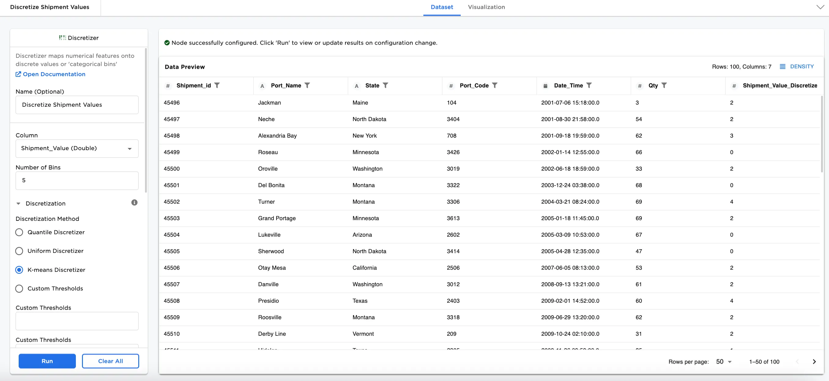
Figure 1: Example output dataframe
Examples
In this example, we have a dataset of shipment information with 100 rows of data. The dataset includes Shipment Ids, Port Names, States, Port Codes, Dates, Qty, and Shipment Values. We'll use this dataset and preprocess it using the Discretizer node for machine learning in the examples. We'll explore all four discretization methods and see how the values are binned differently depending on the method.
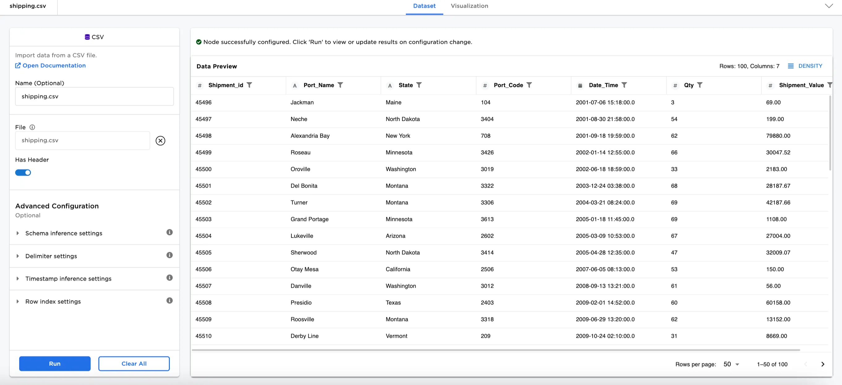
Figure 2: Example input data
- Connect a Discretizer node to an existing node. In this case, it is connected to the Shipment CSV file.
- Optionally, name the Discretizer node. In the example, the node is named,
Discretize Shipment Values. - Select the Column label you'd like to encode. In Figure 3a, the
Shipment_Value (Double)is selected. - Select the Number of Bins. In Figure 3a,
8is entered in the field. - Select a Discretization Method. For this first example,
Quantile Discretizeris selected. - Select the output encoding. Select
Ordinal - Categorical Encoding(default). - Select whether to keep the original column or not. The button is toggled on in Figure 3a.
- Enter a suffix for the discretized column. The default is
_Discretized. - Select Run.
Figure 3a shows the dataframe with a new column at the end of the dataset called, Shipment_Values_Discretized with the original column kept in the dataset. The data in the Shipment_Values_Discretized column is converted into a machine-readable numeric form that represents the number of the bin the value appears in. For example, the third row shows 79880.00/Alexandria Bay is in bin 7.
Selecting the Shipment_Value_Discretized column brings up the metrics for the column. Notice that Figure 3b shows the distribution of values across the eight bins. These metrics represent how the Quantile method distributes the column values into bins. This method shows that the values are close to evenly distributed across the eight bins that are configured.
Notes:
- Bin numbering begins at
0for the first bin, to7for the eigth bin. - Selecting
Non Ordinal - One Hot Encodingencodes the column with a machine-readable numeric value. See Figure 7c and Figure 7d for an example of what this looks like using the selections for Figure 3. Refer to the One Hot Encoding node for more information.
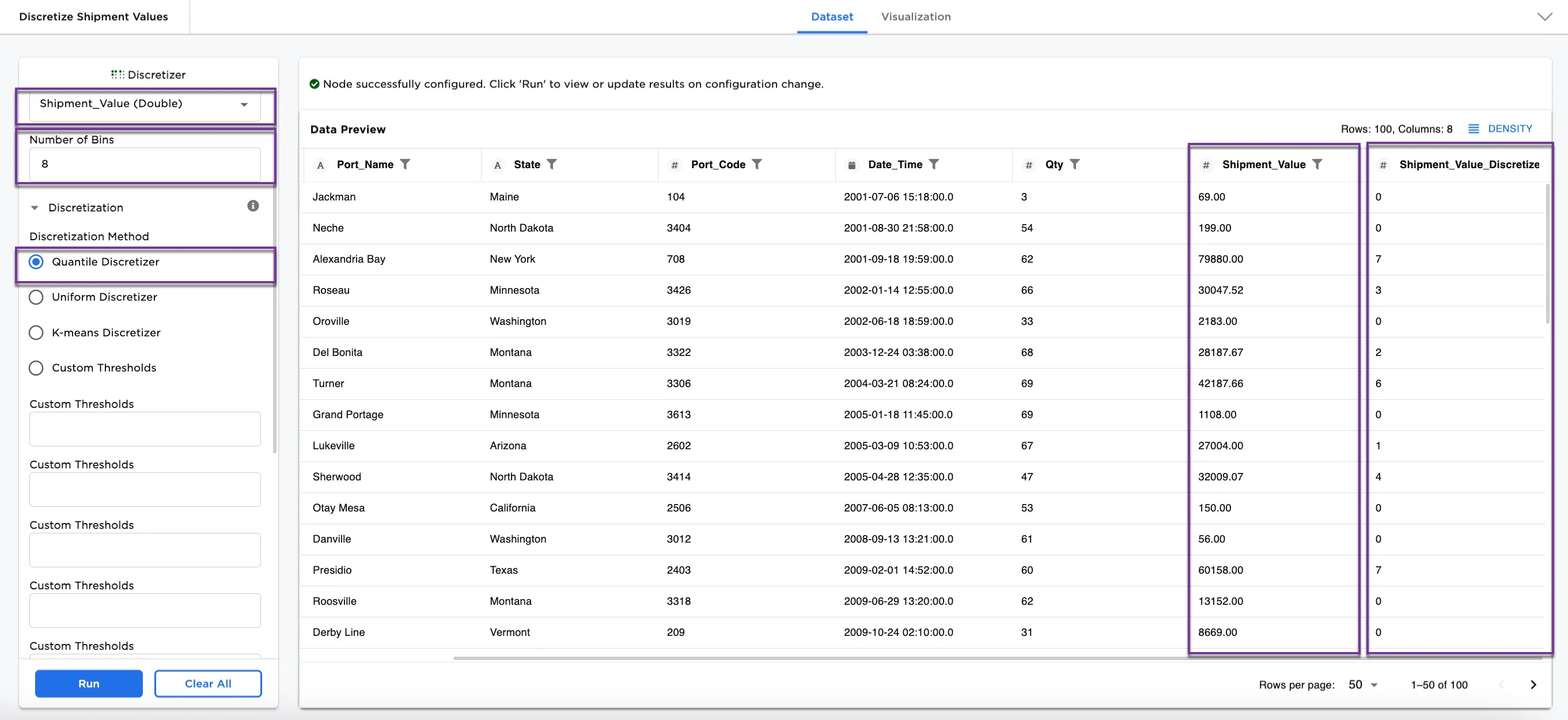
Figure 3a: Example dataframe using the Quantile Discretizer method in 8 bins
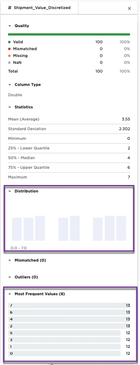
Figure 3b: Example metrics on the Shipment_Value_Discretized column
Optionally, we can also use a different method.
- For Figures 4a and 4b,
Uniform Discretizerhas been selected for the Disrectization Method. - Keep Original Columns is now toggled off.
- Select Run.
Notice in Figure 4a, the third row shows Alexandria Bay in bin 3. The uniform discretizer places the same value in a different categorical bin than the quantile discretizer.
Figure 4b shows the metrics on the Shipment_Value_Discretized column. The bar chart and most frequent values have changed dramatically with this new method. The majority of the shipping values, 83, are in bin 1.
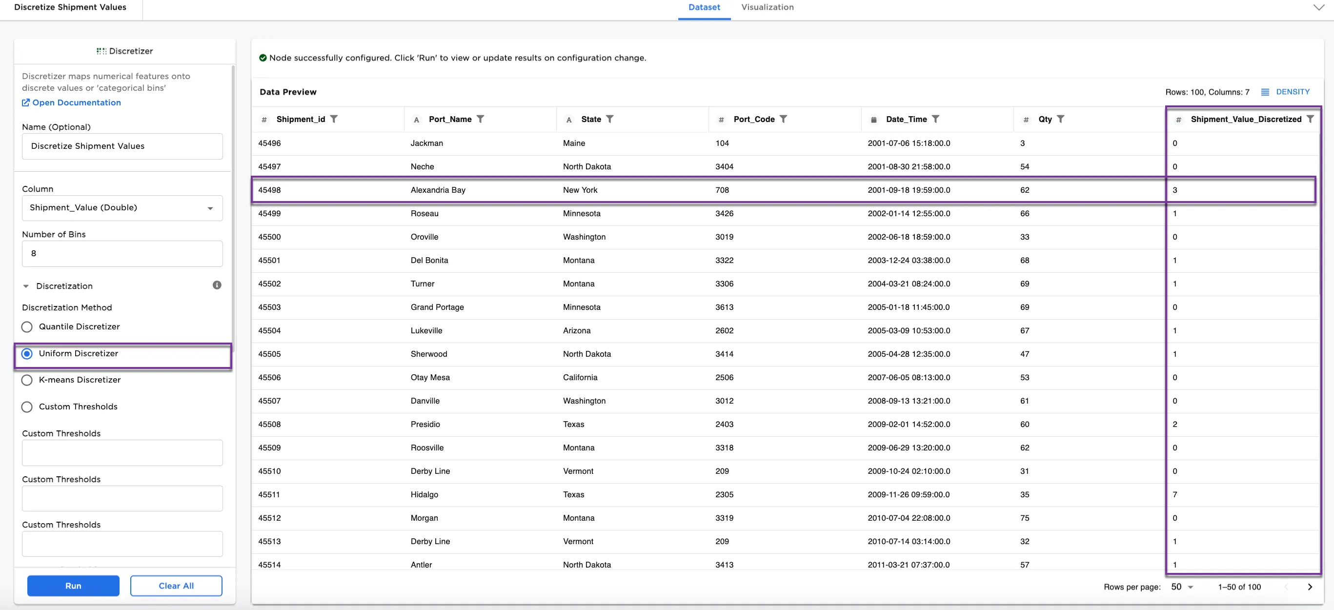
Figure 4a: Example dataframe using the Uniform Discretizer method
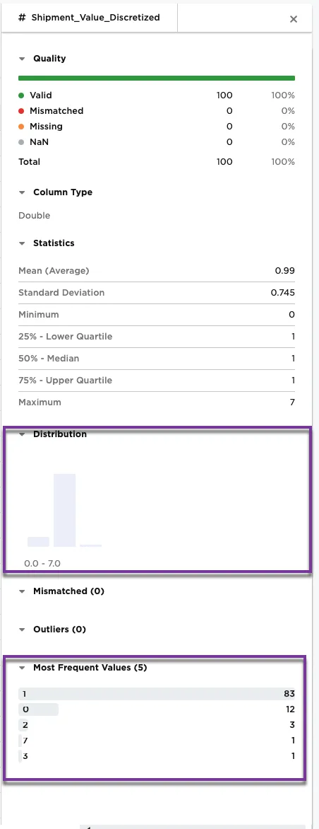
Figure 4b: Example metrics on the Shipment_Value_Discretized column
Another optional discretization method is K-means Discretizer. The K-means discretization method clusters data into a number of clusters, defined by the letter "k," which is fixed beforehand.
- For Figures 5a and 5b,
K-Means Discretizeris selected for the Disrectization Method.
Notice in Figure 5a, the third row shows Alexandria Bay in bin 4.
Figure 5b shows the metrics on the Shipment_Value_Discretized column. The bar chart and most frequent values have once again changed with this new method. Notice that the shipping values are spread throughout the eight bins identified in the configuration.
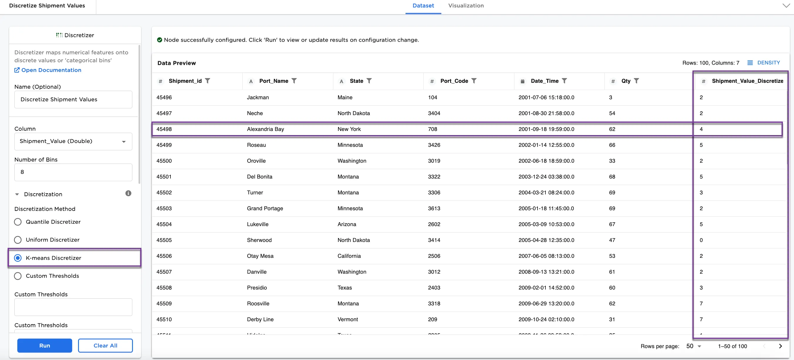
Figure 5a: Example dataframe using the K-means Discretizer method
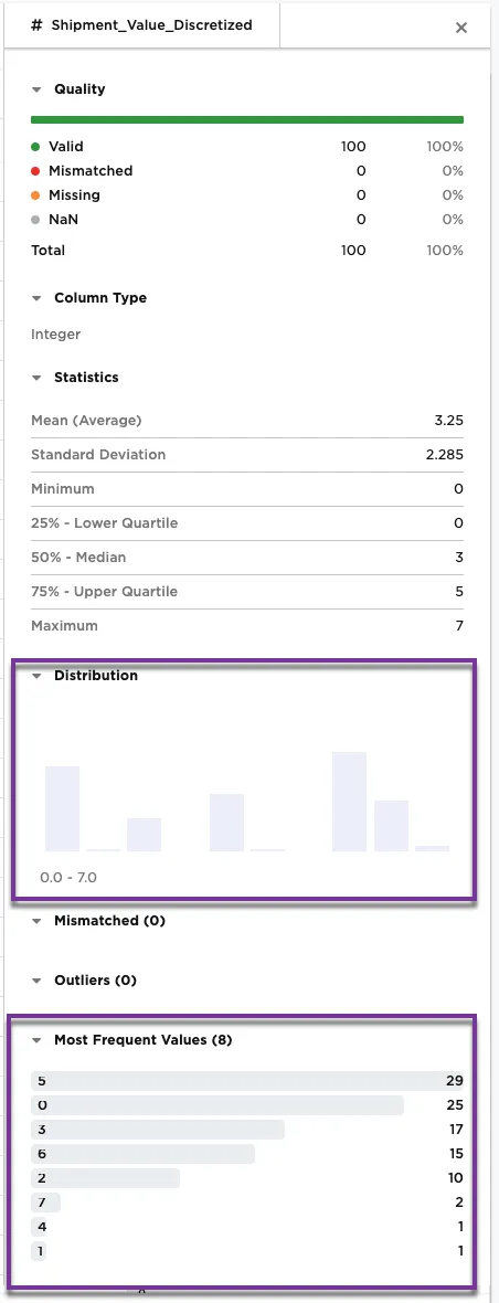
Figure 5b: Example metrics on the Shipment_Value_Discretized column
The last discretization option is the Custom Thresholds method, where you define your own custom thresholds.
- For Figures 6a and 6b, select
Custom Thresholdsfor the Disrectization Method. - In the Custom Thresholds fields, enter
10000,20000,30000,40000, and50000. - For this example, Keep Original Columns is toggled on.
Notice in Figure 6a, the third row shows Alexandria Bay in bin 5. The rows that show 0 are outside of the 10000 to 50000 thresholds entered in the configuration.
Figure 6b shows the metrics on the Shipment_Value_Discretized column. The shipping values are in the bins identified in the Custom Thresholds fields. Notice that there are 14 values outside of the 10000 to 50000 thresholds in the configuration. Notice there are five thresholds defined in the configuration and there are six bins in the metrics. The sixth bin represents the values that fall outside of the five defined thresholds.
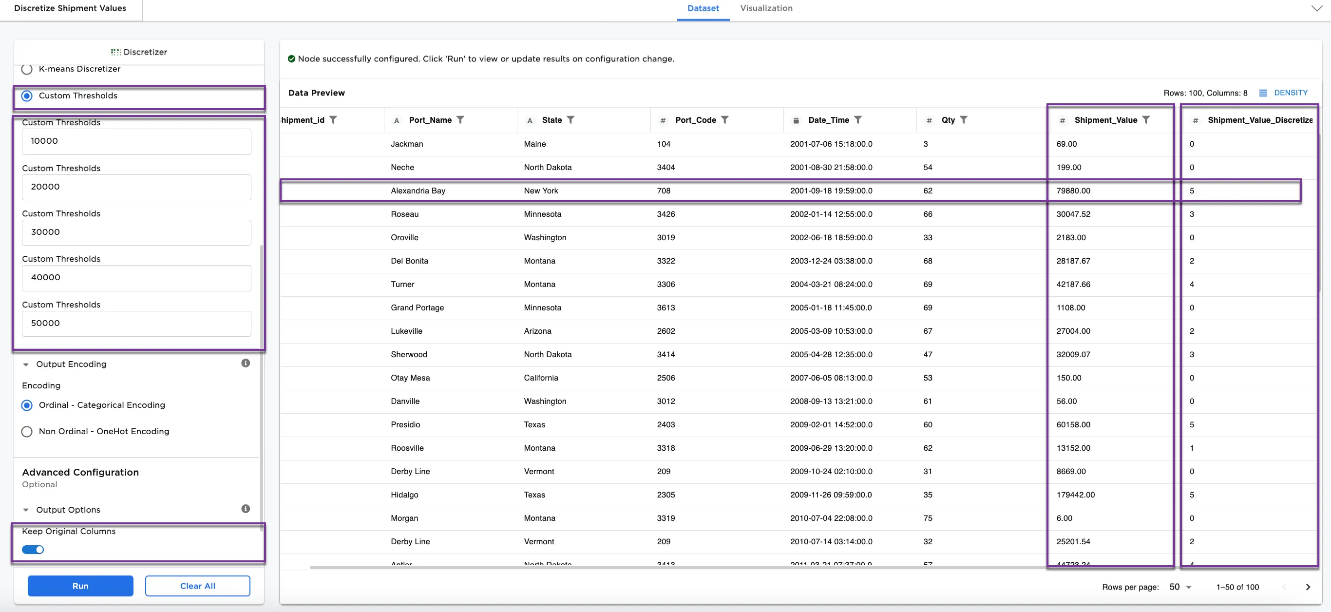
Figure 6a: Example dataframe using the Custom Thresholds method
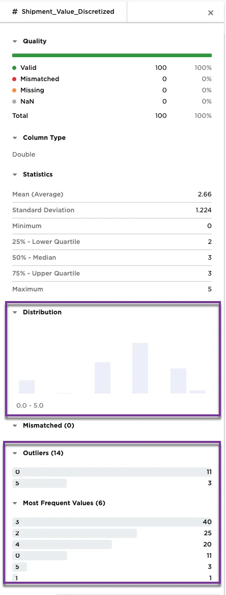
Figure 6b: Example metrics on the Shipment_Value_Discretized column
Thus far, we have used Ordinal - Categorical Encoding. Another option is Non Ordinal - One Hot Encoding. For Figure 7a, change the Encoding to Non Ordinal - One Hot Encoding.
Notice that though the binning has remained the same, the encoding has changed to One Hot Encoding. Instead of a number, the bins are encoded with 0s an 1s, where 1 shows which bin (by position) the shipment value is placed. The third row shows Alexandria Bay with a 1 in the 5th bin position-all other bins show a 0. For more information about One Hot Encoding, see the One Hot Encoding node.
Figure 7b shows the metrics on the Shipment_Value_Discretized column. We are still using the Custom Thresholds discretization method. Notice how the metrics have changed with One Hot Encoding. The six most frequent values represent the 5 threshold bins that have been identified, and the values that do not fall within the bins.
Figure 7c and 7d shows the placement and metrics using Non Ordinal - One Hot Encoding with the Quantile Discretizer and 8 bins (the configurations that we used in Figure 3).
Notice using Ordinal - Categorical Encoding places Alexandria Bay in bin 7 and using Non Ordinal - One Hot Encoding places a 1 for Alexandria Bay in the 4th out of 8 bins. The binning is the same, but the encoding is different. Both types of encoding are suited for preprocessing for machine learning.
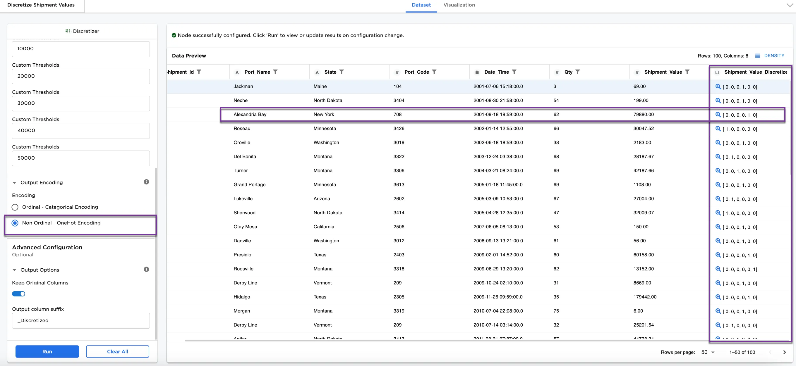
Figure 7a: Example of Non Ordinal - One Hot Encoding
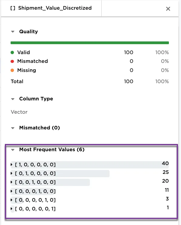
Figure 7b: Example metrics on the Shipment_Value_Discretized column

Figure 7c: Example of Non Ordinal - One Hot Encoding on the Shipment_Value column using the Quantile Discretizer in 8 bins
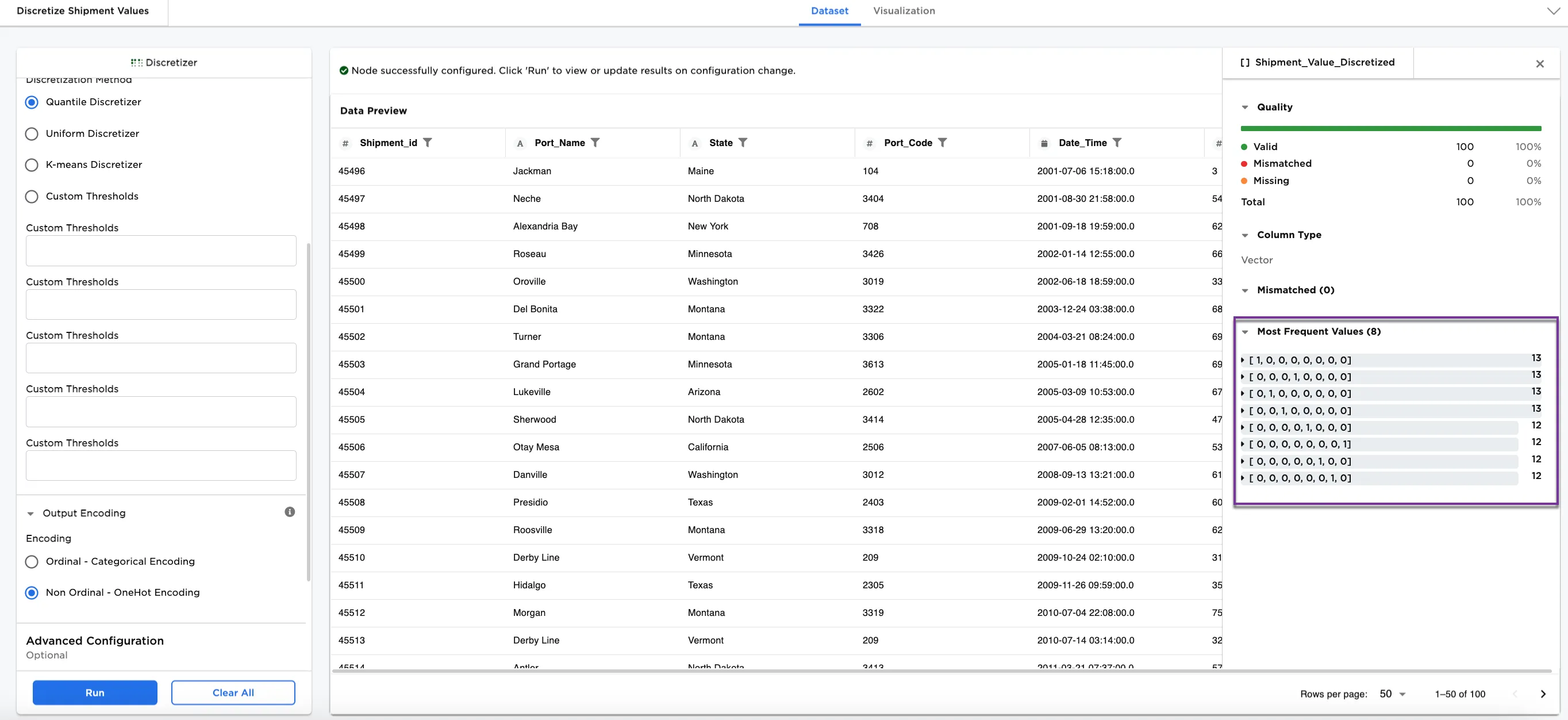
Figure 7d: Example metrics on the Shipment_Value_Discretized column using the Quantile Discretizer method and 8 bins with One Hot Encoding