Data Wrangling and Feature Engineering in Visual Notebooks
Visual Notebooks offers data transformation nodes to perform common data wrangling tasks or analysis tasks such as:
- Describing and profiling data
- Joining data
- Filtering data
- Cleaning data such as imputing missing values
Describe Columns Node for Data Profiling
The first step in many data science projects is to profile and understand the shape and quality of data.
The Describe Columns node is frequently used as a first step in the development of Visual Notebooks visual notebooks and can be used for data quality inspection and general profiling. Capabilities include:
- Profiling missing value and outliers
- Profiling distribution statistics such as mean, quartiles, skew, and kurtosis
- Checking for categorical columns and counting unique values
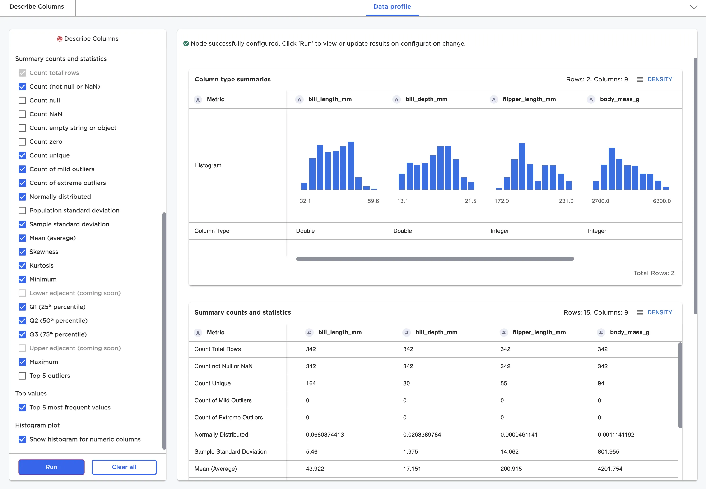
Figure 1: Describe Columns node
Column Profiling
Data at any step in a Visual Notebooks visual notebook can be explored and profiled by simply running the node. Running a node runs the entire visual notebook up to the node undergoing inspection.
Data for a specific node is shown in a tabular grid. Pagination is supported to ensure scalability of the UI. Any column may be filtered and sorted directly within the grid for simple exploration. Columns may be profiled by clicking on a column header to bring up the column summary statistics as depicted in Figure 2. Dedicated timeseries nodes offer the additional profiling ability to generate inline timeseries charts.
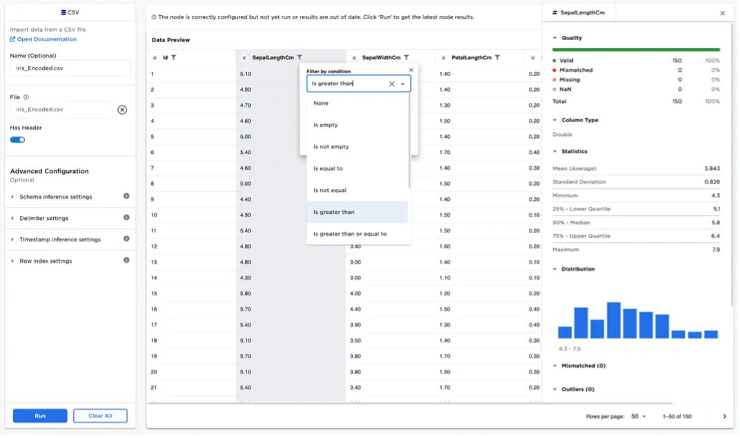
Figure 2: Column data profile for numeric columns
Appending, Joining, and Pivoting Data
Appending/concatenating, joining, and pivoting data are some of the most common data operations for any data science project. Visual Notebooks offers visually rich interfaces for performing these common operations. End users do not need to remember the difference between different join types, as Visual Notebooks guides the user.
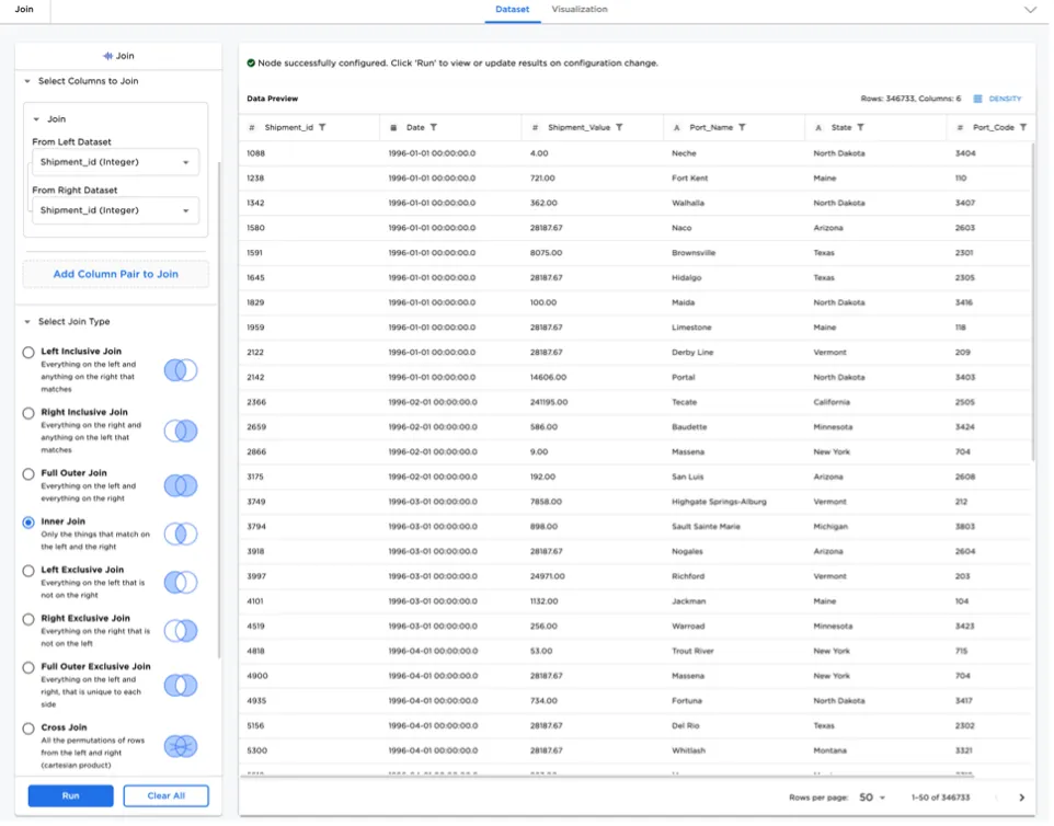
Figure 3: Join node
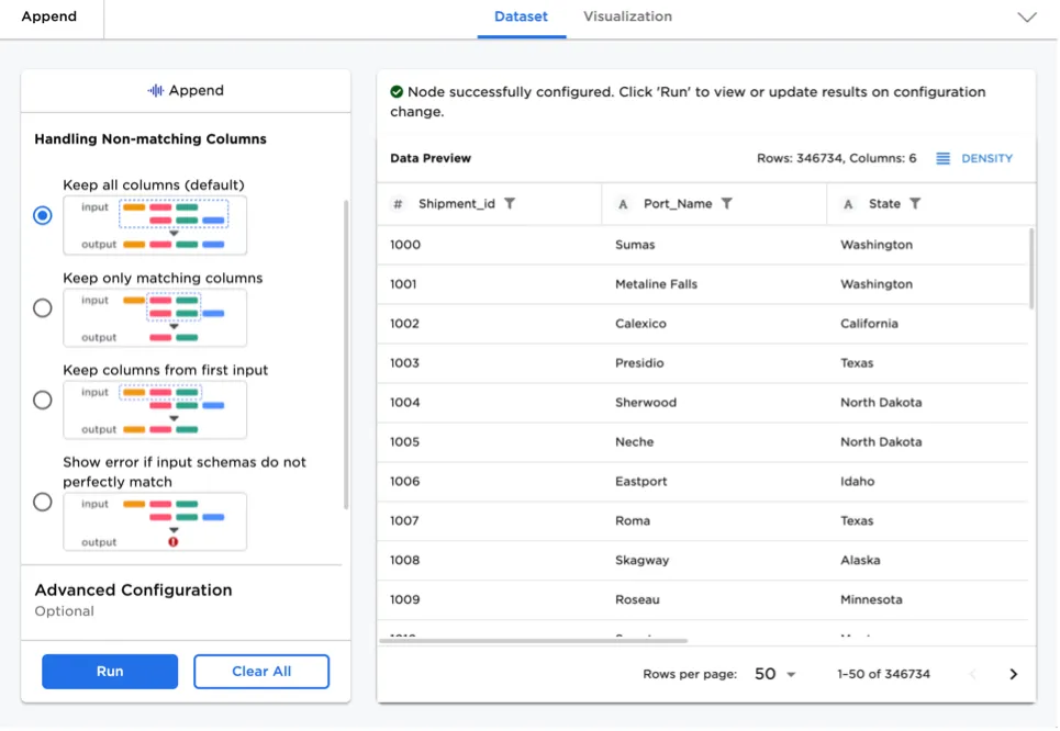
Figure 4: Append node
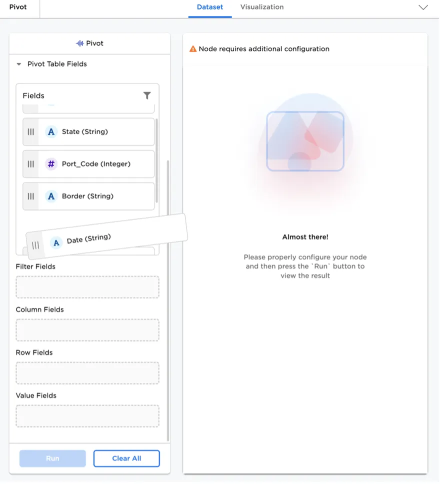
Figure 5: Pivot node with intuitive interface
Wrangling Semi-Structured Data
Often data does not come in a clean tabular format, especially when parsing XML or JSON files. Visual Notebooks offers several transformations for manipulating large semi-structured datasets, including the ability to flatten and explode columns with objects and arrays.
Transformations include:
- Assemble Object
- Assemble Array
- Array Length
- Extract Field from Object
- Extract Value from Array
- Split Object to Columns
- Split Array to Columns
- Explode to Rows (Object or Arrays)
- Flatten Column (Object or Arrays)
- JSON string to Object
The Extract Field from Object node, as an example, enables users to view the schema of a potentially deeply nested object column and select one or more fields to extract
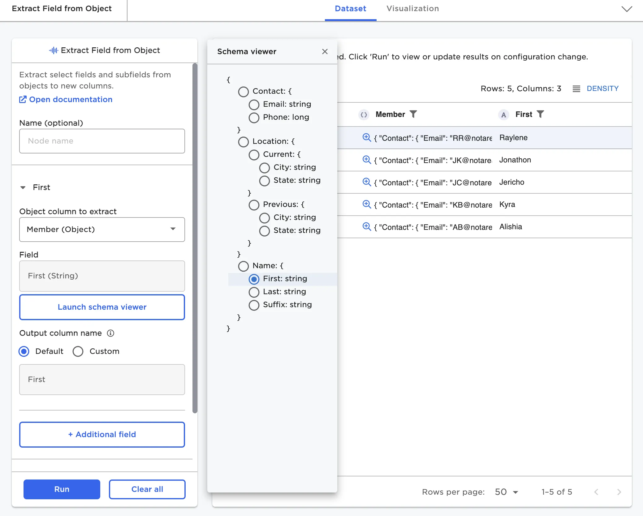
Figure 6: Extract Field from Object node
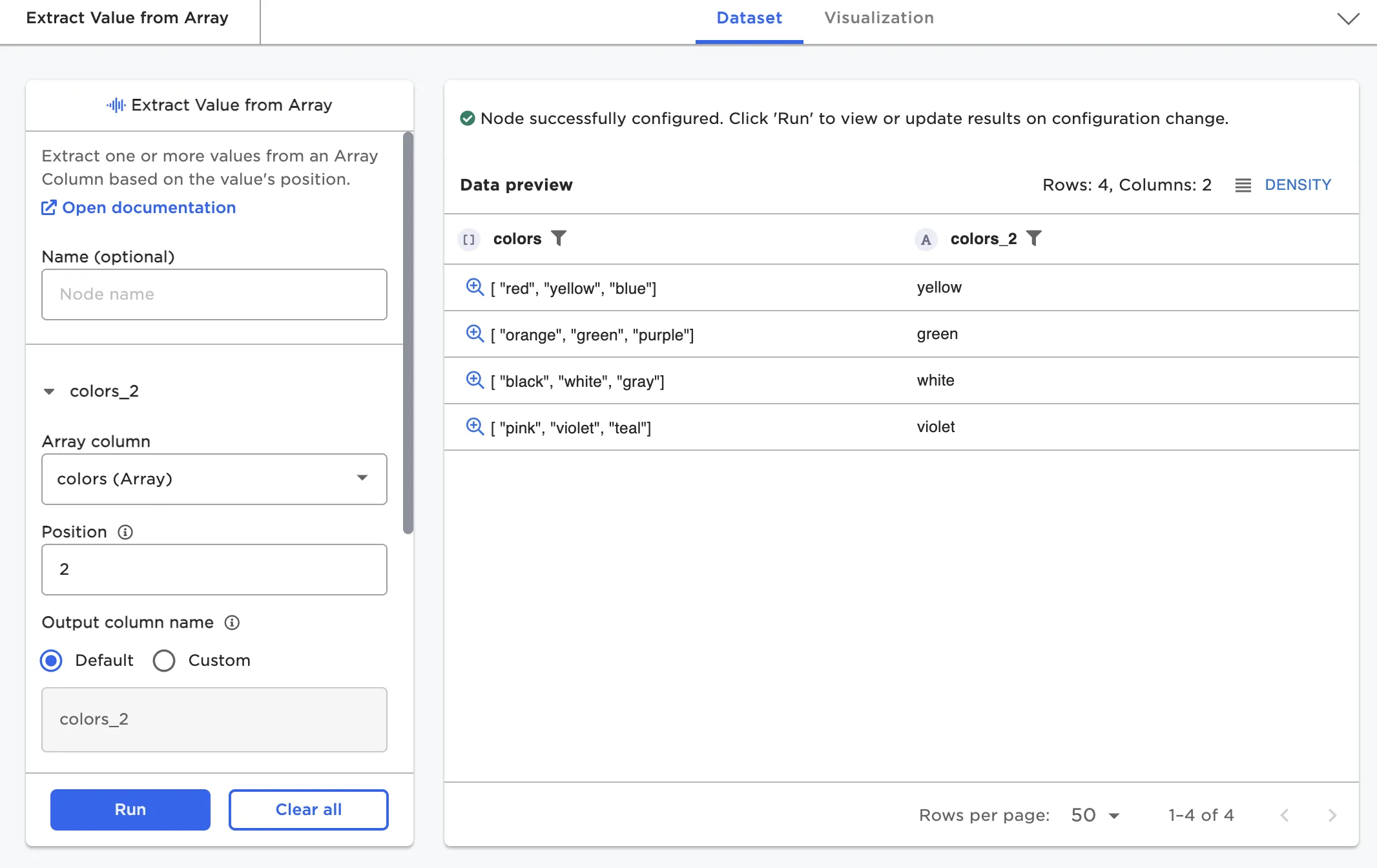
Figure 7: Extract Field from Array node
Timeseries Analysis and Feature Engineering
Timeseries analysis is a cornerstone for many data science projects. C3 AI Ex Machina offers several timeseries manipulation capabilities including the ability to clean timeseries data and generate timeseries features.
Resample and Interpolate
The Timeseries Resample and Interpolate node supports several prebuilt common use cases (downsampling, upsampling, strict interpolation or filling in of missing values, aligning irregularly spaced data). There are also additional options to define custom steps. Selecting a predefined use case will automatically create the sequence of steps (in order) to be performed on the data as pictured in Figure 15.
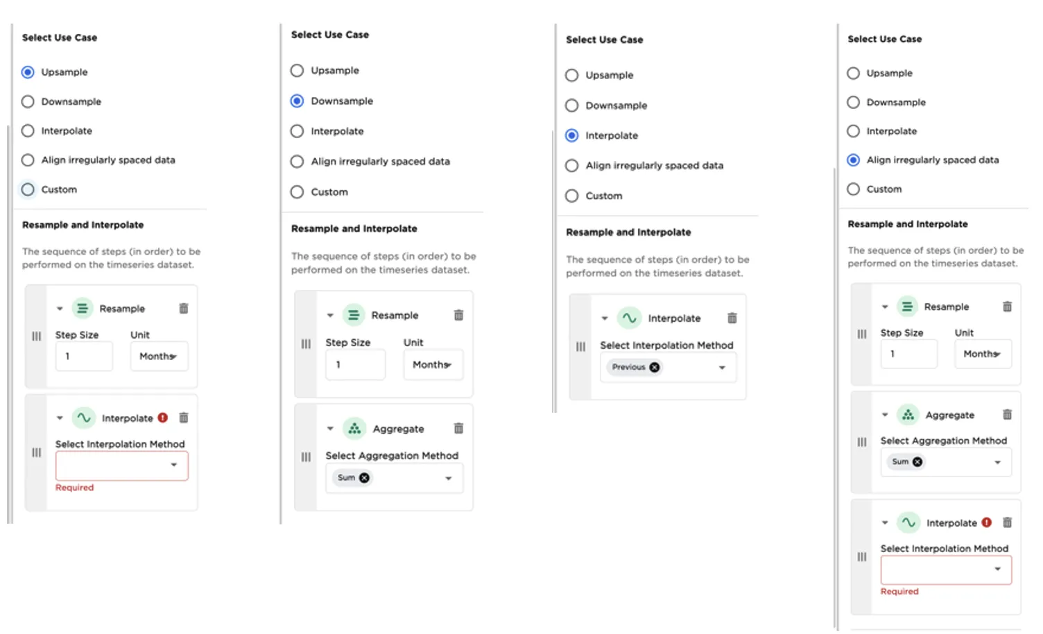
Figure 8: Timeseries Resample and Interpolate use case patterns
Feature Creation
Visual Notebooks timeseries feature engineering nodes simplify the rapid creation of dozens of timeseries features for timeseries-based machine learning. Select examples include:
- Time Extract
- Percent Change
- Shift
- Rolling Window
- Rolling Cumulative Aggregate
The Rolling Window node, as an example, allows the creation of many window features with a single click. Users may simultaneously select multiple columns, multiple functions, and multiple windows. A cross product of the columns, functions, and windows will result in dozens or hundreds of new features. Each feature is added and labeled as a new column with the nomenclature window_function_colname.
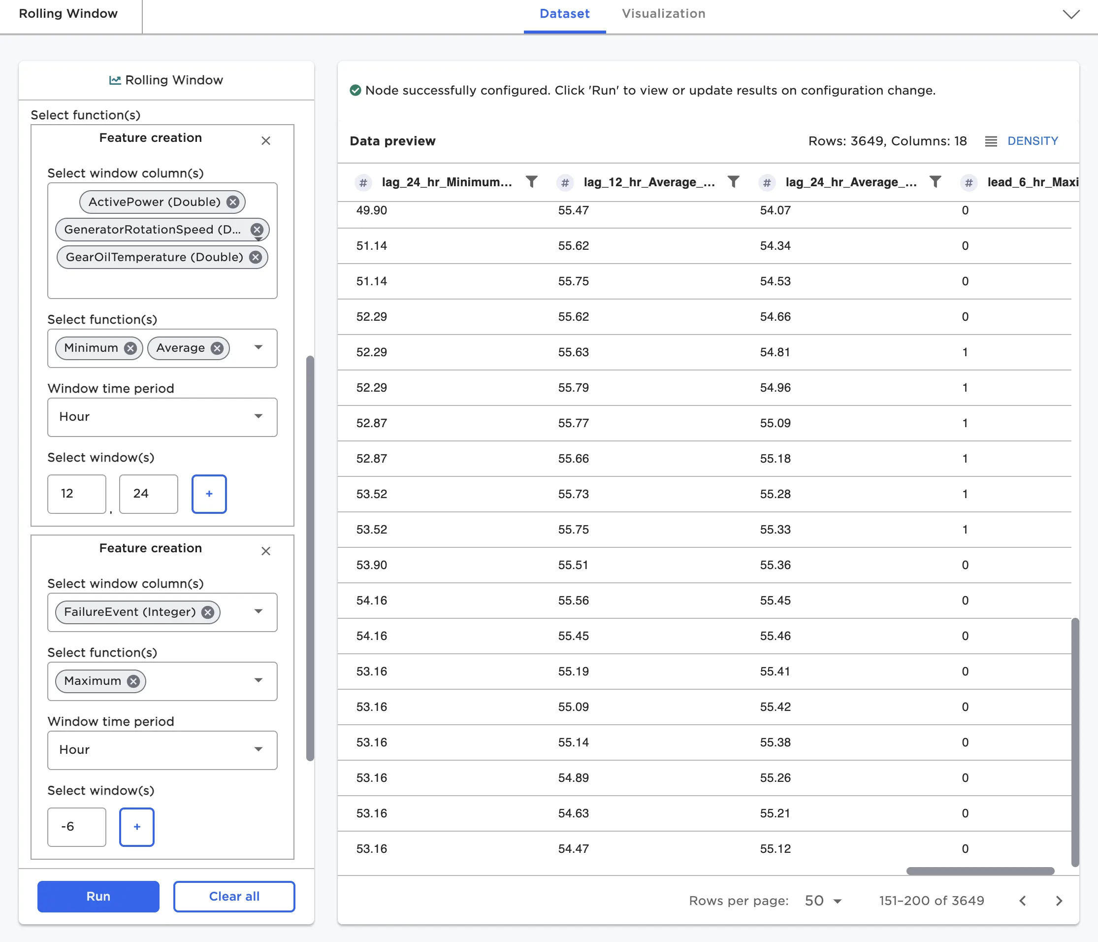
Figure 9: Rolling Window node configuration
Statistical Analysis
Statistical analysis is an important tool in many data science projects. Visual Notebooks offers several nodes that enable single-sample and multiple-sample hypothesis tests. When combined with statistics charts such as box plots and QQ plots, these nodes enable a wide variety of use cases including:
- Marketing A/B Testing
- Quality control and manufacturing process control testing and analysis
- Pharmaceutical trial analysis of control vs. experimental groups
Each statistics node helps with framing a specific test as a hypothesis, with details on test statistic and confidence interval assumptions.
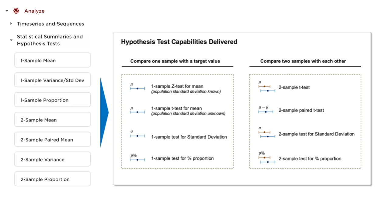
Figure 10: List of supported statistics nodes and available tests
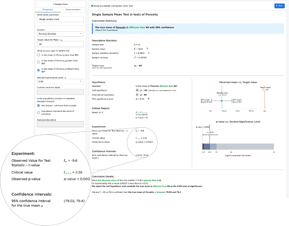
Figure 11: Example Statistical Test
Freeform Expressions: Arithmetic, Custom SQL Function, Python Notebook
Often it is necessary to perform complex row or column operations. Visual Notebooks offers a variety of "free form" nodes to provide flexibility including:
- Column arithmetic node
- Custom SQL expression node
- Python notebook node
The Arithmetic node allows users to perform complex expressions across columns without needing to know any SQL or Python. A calculator-like interface is provided allowing users to select and combine columns and functions.
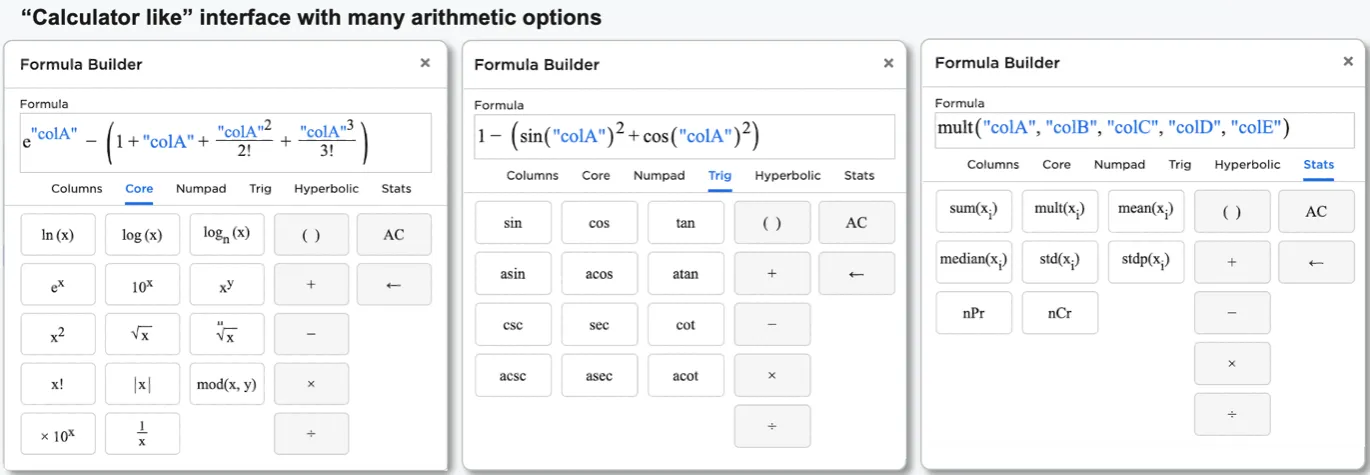
Figure 12: Arithmetic node
The Custom SQL expression node allows users to perform any Spark SQL operation on a dataframe. A list of available columns is provided. The user must "evaluate and save" the SQL expression to ensure it is valid before running the node.
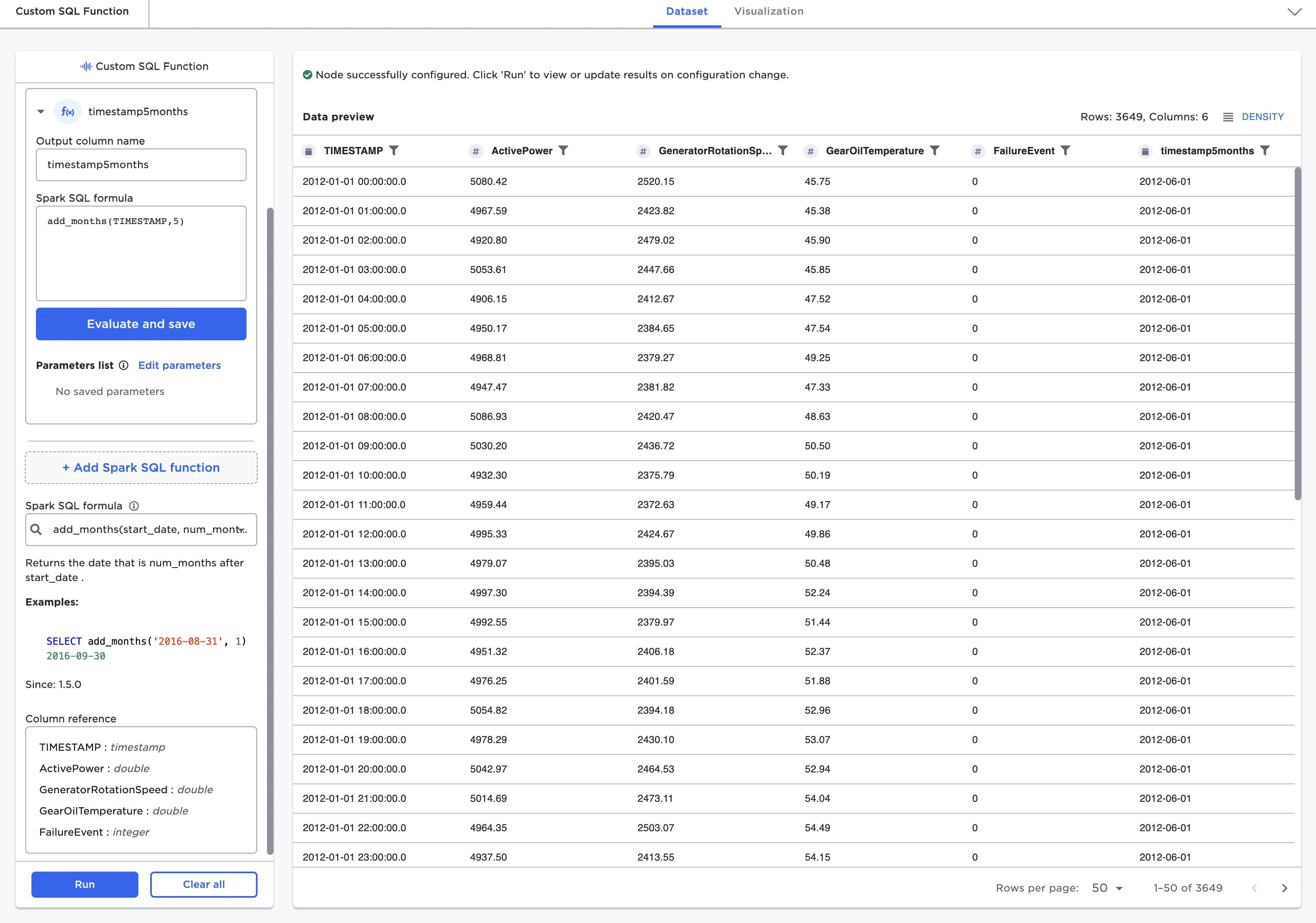
Figure 13: Custom SQL node
The Python node (in private beta with customers) allows users to write any abstract "py-spark/pandas on spark" code snippet. It can be thought of as injecting a single notebook paragraph into the visual notebook flow. The full py-spark library is available to this node.
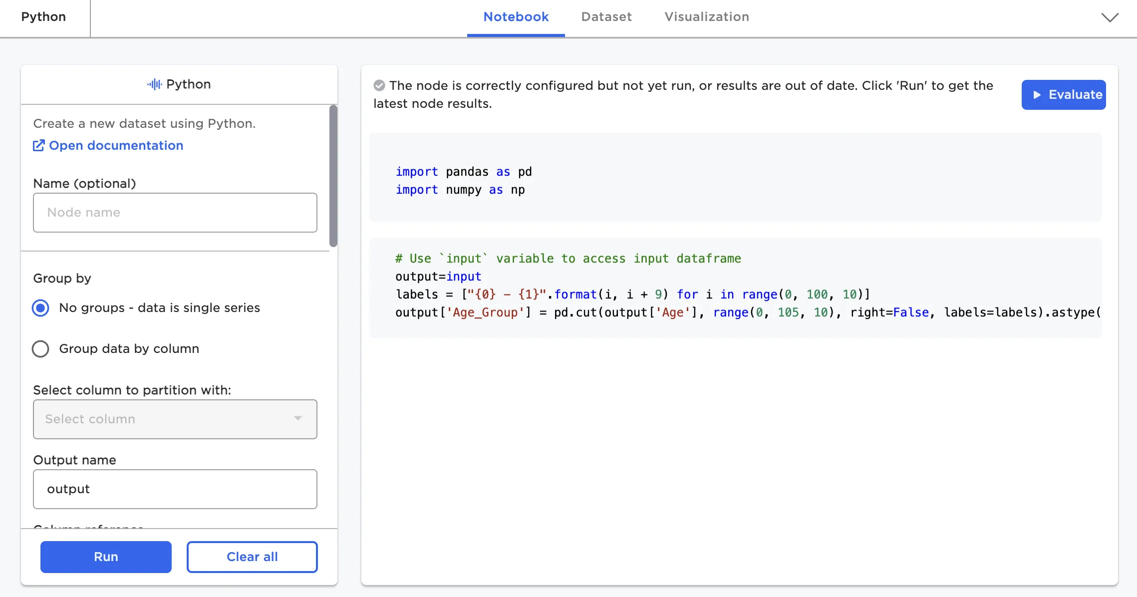
Figure 14: Python node