Percent Change
Calculate how values change over time using the Percent Change node in Visual Notebooks.
The percentage change is used to analyze and compare data over time and percentage points. It is particularly helpful to analyze differences in rates of change.
Configuration
| Field | Description |
|---|---|
| Name default=none | Name of the node A user-specified node name displayed in the workspace, both on the node and in the dataframe as a tab. |
| Column with Timestamps or Sequence (x axis) Required | Columns with values Select a column with timestamps (or numeric data) from the dropdown menu to track percent change over time. The column selected for this field should should contain timestamps or numeric data. |
Group by default=No groups - data is single series | Grouping selection Select whether to view the data in a single series or grouped by data in another column. |
| Select column to partition with: default=none | Column to group by If Group data by column is selected for the Group by field, select a column to partition the data. |
| Select Percent Change Column(s) Required | Select column(s) to view percent change Select columns with data to analyze the percent change over time. |
| Select Lag Offset(s) Required | Enter lag offset Enter the positive or negative factor to calculate the percent change over entries in the timeseries or sequence. A positive integer calculates the percent change with the value before the selection (lag) and a negative integer calculates the percent change with the value after the selection (lead). "1" as the factor represents percent change one value before the other in the timeseries or sequence; "3" as the factor represents the percent change over three earlier values in the timeseries or sequence; "-2" as the factor in comparison, represents the percent change over two subsequent values after the selection. |
Node Inputs/Outputs
| Input | A Visual Notebooks dataframe |
|---|---|
| Output | A dataframe with additional percent change columns |
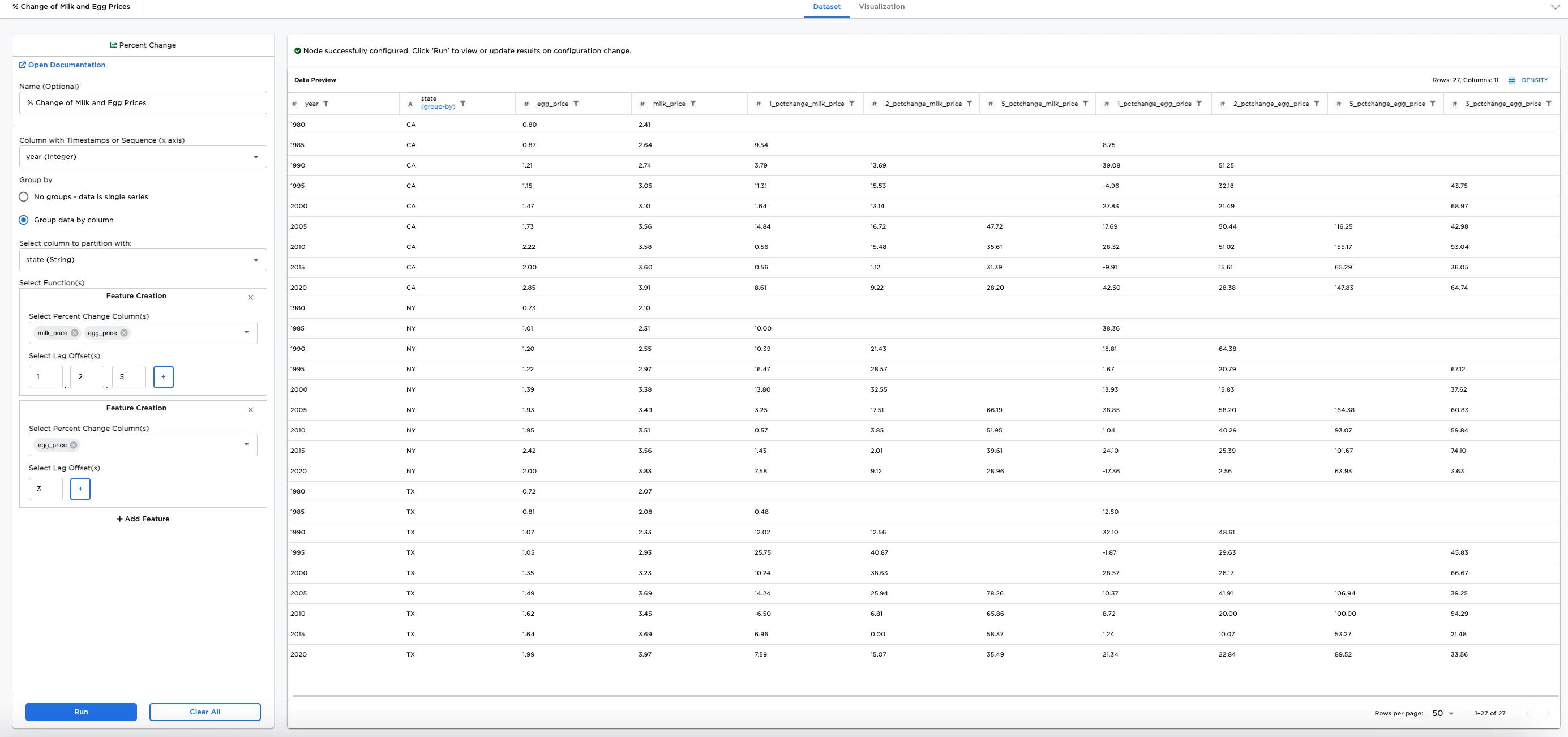
Figure 1: Example output
Examples
During times of inflation or deflation, it can be useful to analyze the percent change in prices over time. Let's say you want to analyze and compare the percent change of the price of milk and eggs over time from one state to another. First, you'll need to start with a dataset that contains the pricing information for these items in different states over a period of time. The dataframe shown in Figure 2 contains data about the price of milk and eggs in three US states from 1980 to 2020.
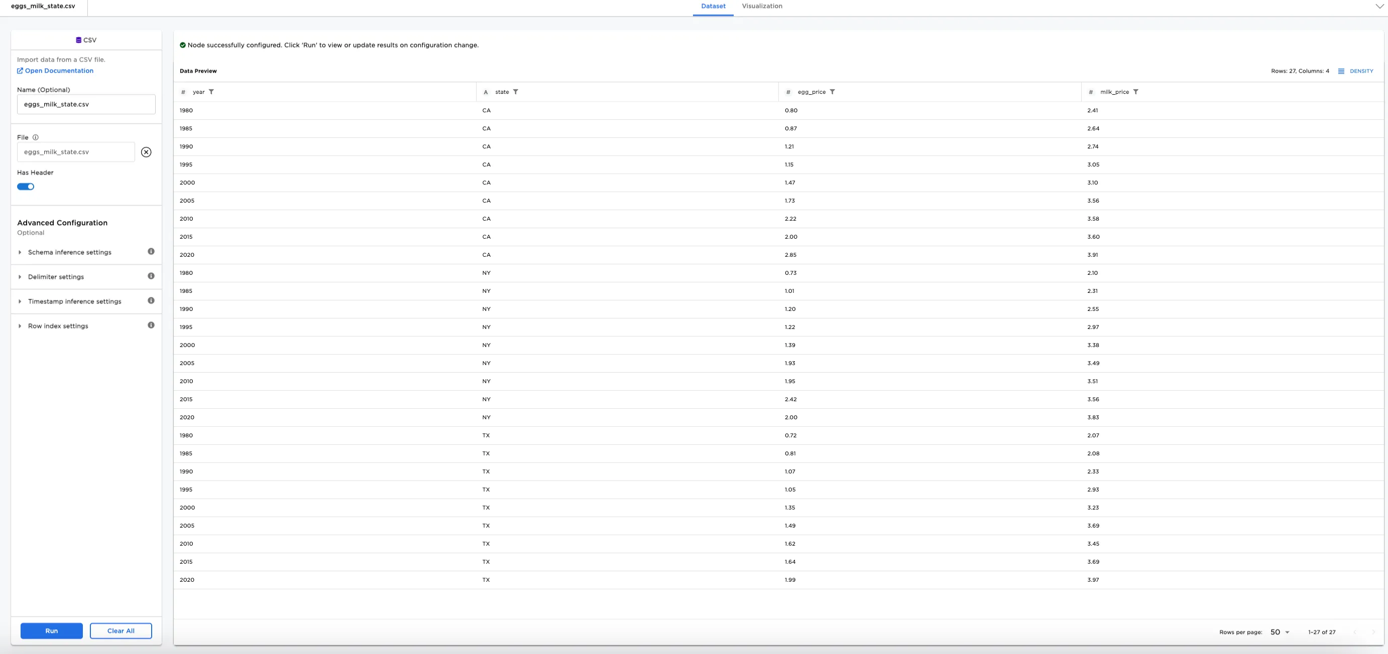
Figure 2: Example input data
The following are definitions for important percent change fields used in this node:
- Column with Timestamps or Sequence (x axis) field: A timestamp column is ideal to calculate the percent change over time periods, but if your data does not have a timestamp column, selecting another column with another ordering system (month 1, month 2, for example) also works. If a numeric field is selected, Visual Notebooks orders the data in the field in sequence (values are represented from lowest to highest).
- Lag Offset field: Entering "1" for the lag offset compares each successive price to the previous price to calculate the percentage. Comparing the price from one year to the prior year might show a lower percent increase or decrease. Entering "3" calculates the percent change from the price three values prior in the time or sequence. Comparing the price from a year to three years prior might show a higher percent increase or decrease.
- Connect a Percent Change node to an existing node. In this case, it is connected to a CSV node with the "Eggs_Milk_State" file.
- Optionally, name the Percent Change node. In the example, the node is named, "% Change of Milk and Egg Prices."
- Select the Column with Timestamps or Sequence (x axis) field. Figure 3 shows
year (integer)selected for this field. - Make your Feature Creation selections. In the example,
milk_priceis selected for the Select Percent Change Column(s) and "1" is entered for the Select Lag Offset(s) field.
Notice Figure 3 includes a new column called 1_pctchange_milk_price and a "group by" suggestion is added to the state column label.
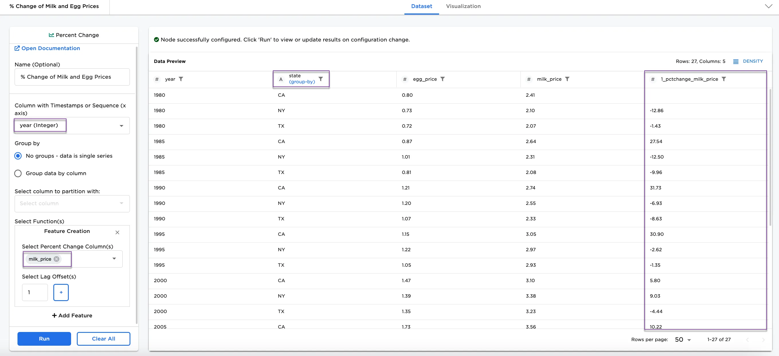 Figure 3: Example of milk price over time
Next, group the data by state:
- Select Group data by column
- In the Select column to partition with: dropdown menu, select
state (String).
Notice that the 1_pctchange_milk_price column shows the price of milk grouped by the state column year over year.
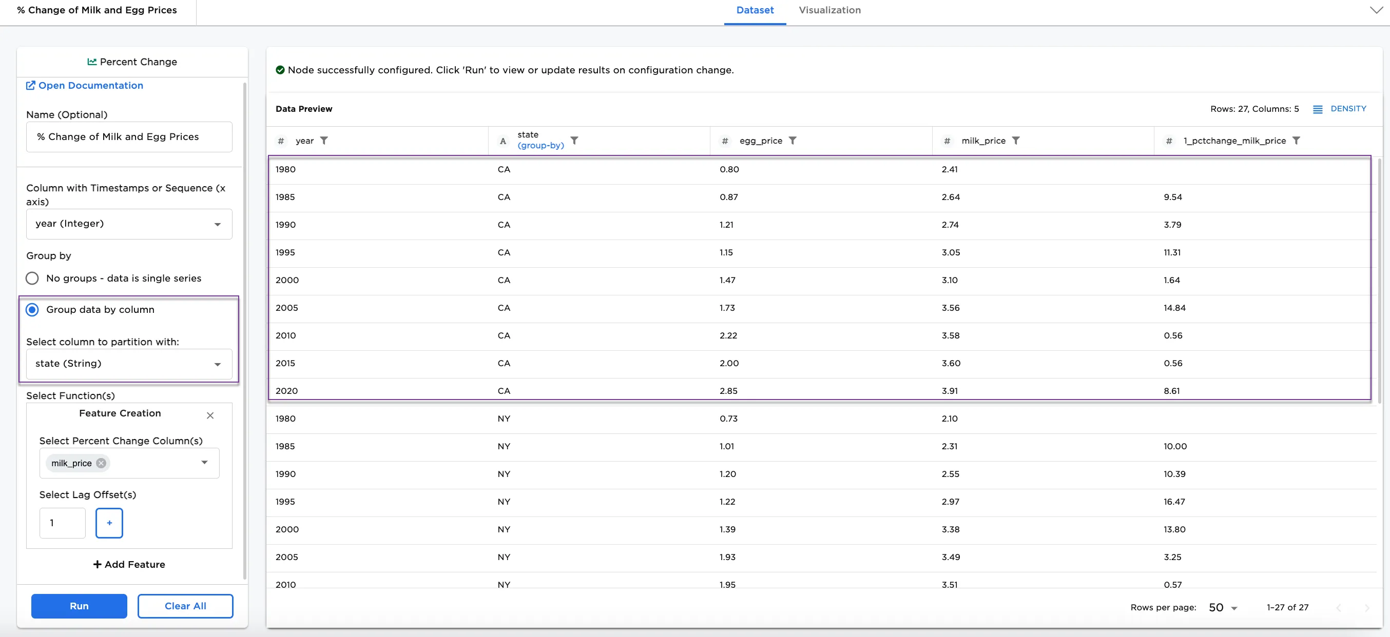 Figure 4: Example grouped by state
Optionally, you can add another column to view and compare percent change over time. In Figure 5, egg_price is added to the Select Percent Change Column(s). Notice that a new column is created called, 1_pctchange_egg_price.
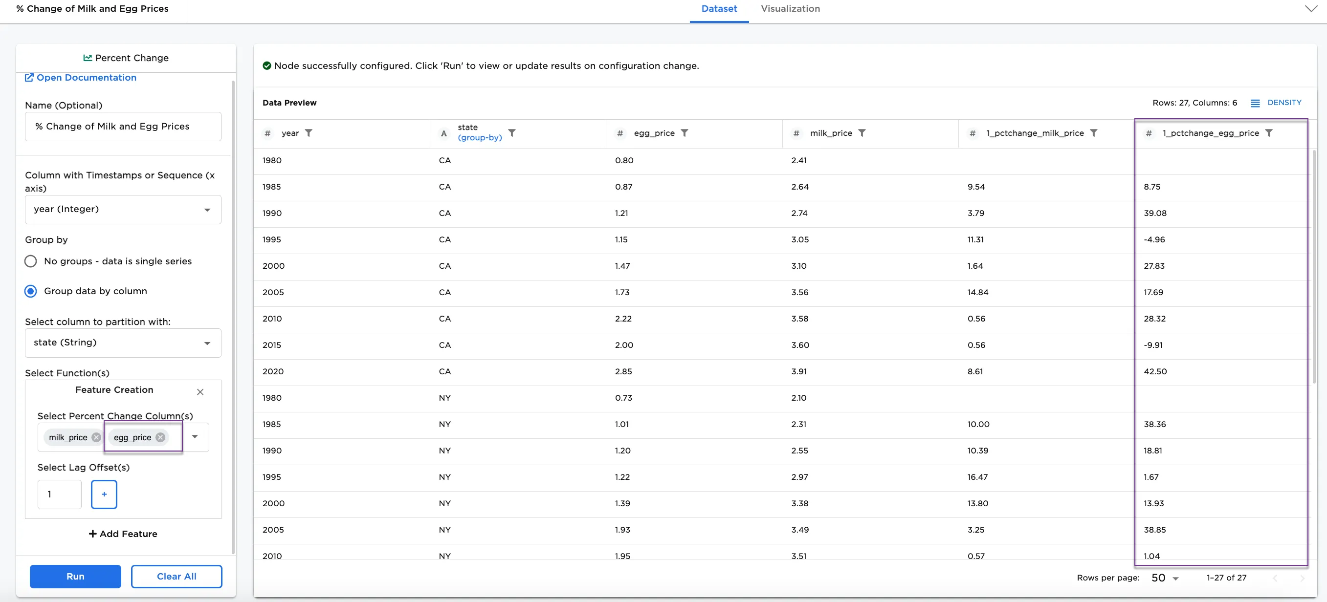
Figure 5: Example selecting two percent change columns
To see more features of this node, try adding these optional selections:
- Select Lag Offset(s): 1, 2, and 5
- Select Percent Change Column(s):
egg_price - Select Lag Offset(s): 3
Notice that there are three new columns showing 1, 2, and 5 for lag offset to calculate the percent change in price for milk, and the same columns showing the percent change in price for eggs, all grouped by state. An additonal column is added that shows only a 3 lag offset for the percent change in price for eggs.
Looking at the 5_pctchange_milk_price column, the first value is 47.72. This shows the percent change of the milk price from 1980 to 2005. Each subsequent row shows percent change of milk price over the five previous years.
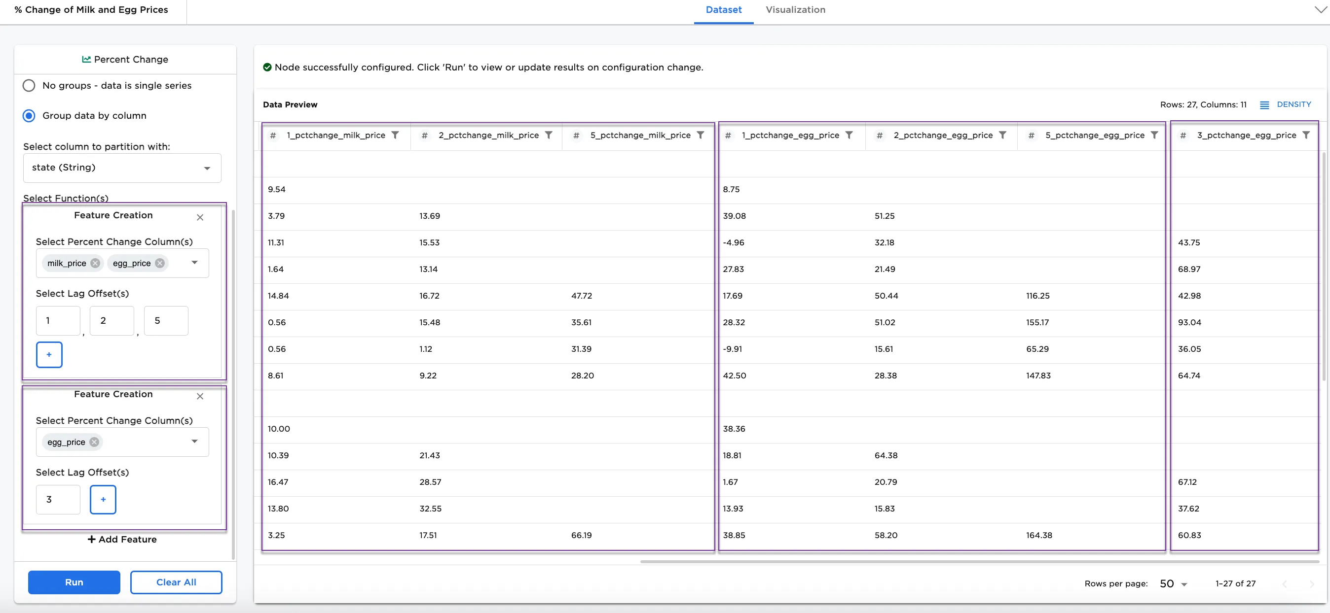
Figure 6: Example with multiple lag offsets