Prophet
Forecast timeseries data using the fbprophet library in Visual Notebooks. Prophet is an additive regression model. This means that the model is simply the sum of different components such as linear or non-linear trend, seasonality and holidays or special events. It is a good choice for timeseries containing strong seasonal effects and several seasons of historical data. Prophet can accommodate missing data and changes in the trend, and usually handles outliers well.
Prophet can be considered a nonlinear regression model of the form:
$y(t) = g(t) + s(t) + h(t) + \epsilon_t$
Here $g(t)$ is the trend function which models non-periodic changes in the value of the timeseries, $s(t)$ represents periodic changes (e.g., weekly and yearly seasonality), and $h(t)$ represents the effects of holidays which occur on potentially irregular schedules over one or more days. The error term $\epsilon_t$ represents any idiosyncratic changes which are not accommodated by the model.
Configuration
| Field | Description |
|---|---|
| Name default=none | Name of the node AA user-specified node name, displayed in the canvas and in the dataframe as a tab. |
Select Input Columns
| Field | Description |
|---|---|
| Column with groups default=none | Column to group data by Select a column as an index to partition your data. A separate forecasting model is built for each resulting dataset. |
| X-axis Required | Column with timestamps Select the column containing timestamps for the values being predicted. Duplicate timestamps must be treated first using Overlapping Data Points under Advanced Configuration. |
| Y-axis Required | Column with values to predict Select the column containing the values to predict. |
Forecasting
| Field | Description |
|---|---|
| Number of Periods Forward to Predict Required | Out-of-sample prediction periods Specify the number of future periods the fitted forecasting model should make predictions on. This time period begins after the latest date in the historical data used for training. |
| Forecast Granularity Required | Timescale for out-of-sample prediction period Select the timescale corresponding to Number of Periods Forward to Predict. |
Testing Strategy
The testing strategy informs the cross-validation process, which is used to determine the set of hyperparameters that produce the best forecasting model. In a classic regression or classification problem, cross-validation involves the random partitioning of training and validation datasets (i.e., creating a fold) to measure training performance. This process is repeated several times, with results averaged to generate the final performance metrics. This approach does not work in the case of timeseries data because it ignores the temporal components inherent in the data.
In Prophet, the first fold is created using a specified initial period for training, and a specified forecast horizon for validation. Training periods in successive folds are created by adding a specified walk forward period (i.e., an expanding window) to the prior training period. This process continues until the range of the combined training and walk forward period exceeds that of the input data. Forecasts made during cross-validation are referred to as simulated historical forecasts (SHFs).
| Field | Description |
|---|---|
| Initial Training Period Required | Period to generate first simulated historical forecast Enter a positive integer and select the corresponding timescale. The period starts from the oldest timestamp, and should be chosen to capture the trend, seasonality and cyclicality of the input data. The larger the period, the greater the weight placed on older data during cross-validation. |
| Walk Forward Period Required | *Period between successive simulated historical forecasts * Enter a positive integer and select the corresponding timescale. The greater the period, the fewer the number of SHFs and therefore the shorter the computation time for cross-validation. However, there will be fewer observations of forecasting errors on which to base model selection. The smaller the period, the greater the number of SHFs and the more correlated their estimates of error are. As a heuristic, Prophet defaults to a period equal to half the Forecast Horizon. |
| Forecast Horizon Required | Forecast period for cross-validation Enter a positive integer and select the corresponding timescale. The horizon should be informed by business requirements (e.g., number of days, weeks, or months of product sales that should be forecast), and is typically the same as Number of Periods Forward to Predict in the Forecasting section. |
Advanced Configuration
Optionally alter the advanced configuration fields to control the output of the node.
Change Points
It can be challenging to model abrupt changes in a timeseries so that trend changes are captured without overfitting the data. Prophet automatically detects these changepoints to appropriately model the trend, but there are several arguments you can use to exert finer control over the process. This is particularly useful if, for example, Prophet missed a rate change, or is overfitting rate changes in the history. A rate change is defined as the change in two values of a timeseries divided by the associated time period (e.g., accelerating from 20 m/s to 40 m/s in 5s represents a rate change of 4 m/s^2).
Prophet first distributes a large number of potential changepoints uniformly across part of the timeseries. It then applies a penalty inversely proportional to the magnitude of the rate changes so that smaller rate changes are ignored. This has the effect of using as few of the changepoints as possible, which prevents overfitting.
| Field | Description |
|---|---|
Number of Changepoints default=25 | Number of potential trend changepoints Enter an integer greater than or equal to zero. This is the number of automatically placed changepoints. |
Change Point Range default=80% | Percentage of timeseries over which changepoints are placed Move the slider to set the proportion of the history in which the trend is allowed to change. This defaults to 0.8, 80% of the history, meaning the model will not fit any trend changes in the last 20% of the timeseries. Changepoints are uniformly placed in this range. |
Saturating Forecasts
Prophet allows either a linear model or logistic growth model to be selected for its trend function, $g(t)$, which models non-periodic changes in the value of the timeseries.
A linear model is selected by default. Linear models allow the trend to increase or decrease without limits. Forecasting problems involving growth (e.g., total population size or total market size) have an upper limit that make linear models unsuitable. In a logistic growth model, this is called the carrying capacity, and the forecast should saturate (i.e., reach an asymptotic limit) at this point.
| Field | Description |
|---|---|
Select Growth Type default=Linear | Choose trend function Select Linear or Logistic. If Logistic is selected, enter an integer for the Cap (i.e., carrying capacity) and Floor. The floor is the saturating minimum. The logistic function has an implicit minimum of 0, and will saturate at 0 the same way that it saturates at the capacity. |
Uncertainty Interval
Uncertainty in the forecast trend is measured by assuming that the future will see the same average frequency and magnitude of rate changes that were seen in the history. Rate changes are computed using the changepoints created in the Change Points section, and their distribution is used to generate future changepoints through random sampling. This generative model is used to simulate possible future trends, which are used to compute uncertainty intervals.
Uncertainty intervals are a useful indication of the level of uncertainty, and especially an indicator of overfitting. As changepoint_prior_scale in the Hyperparameters section (note: the Hyperparameters section is currently under development) is increased the model has more flexibility in fitting the history and so training error will drop. However, when projected forward this flexibility will produce wide uncertainty intervals, an indication of overfitting.
| Field | Description |
|---|---|
Interval Width default=80% | Width of uncertainty interval Enter an integer between 0 and 100. Prophet returns uncertainty intervals for each component, with lower and upper bounds labeled yhat_lower and yhat_upper, respectively, in the dataset table. The forecast is labeled yhat. These are computed as quantiles of the posterior predictive distribution (i.e., the distribution of values predicted by the model over the input timeseries), and Interval Width specifies which quantiles to use. The default provides an 80% prediction interval. Changing the width will affect only the uncertainty interval. It will not change the forecast yhat at all and so does not need to be tuned. |
Holidays
Holiday effects can be modeled and included in the forecast. They will also show up in the components plot.
| Field | Description |
|---|---|
Select Country default=None | Country with holidays to use Select a country from the dropdown menu to apply a built-in collection of country-specific holidays. |
Seasonality
Prophet uses additive seasonalities by default. This means the forecast is computed by adding the seasonality to the trend. In some cases, the seasonality is not a constant additive factor, but rather grows with the trend. This is multiplicative seasonality. This type of seasonality is best identified by looking at the timeseries and seeing if the magnitude of seasonal fluctuations grows with the magnitude of the timeseries. If it isn't possible to tell, you can train separate models (one with additive seasonality and the other with multiplicative seasonality) and select the seasonality type that results in better performance.
| Field | Description |
|---|---|
Select Seasonality Mode default=Additive | Impact of seasonality Select Additive for additive seasonality, or select Multiplicative for multiplicative seasonality. |
Overlapping Data Points
For timeseries data in Visual Notebooks, overlapping data points refers to data with one or more duplicate timestamps. In most cases, if this data is not aggregated, results will be inaccurate or worse, the analysis altogether cannot be performed. The field in this section provides options for aggregating the data.
| Field | Description |
|---|---|
Treatment default=Average | Aggregation methods Select an aggregation function from the dropdown menu. Available options are Average, Sum, Minimum, Maximum and Count. |
Node Inputs/Outputs
| Input | A Visual Notebooks dataframe |
|---|---|
| Output | Trained Prophet forecasting model and a dataframe with predictions |
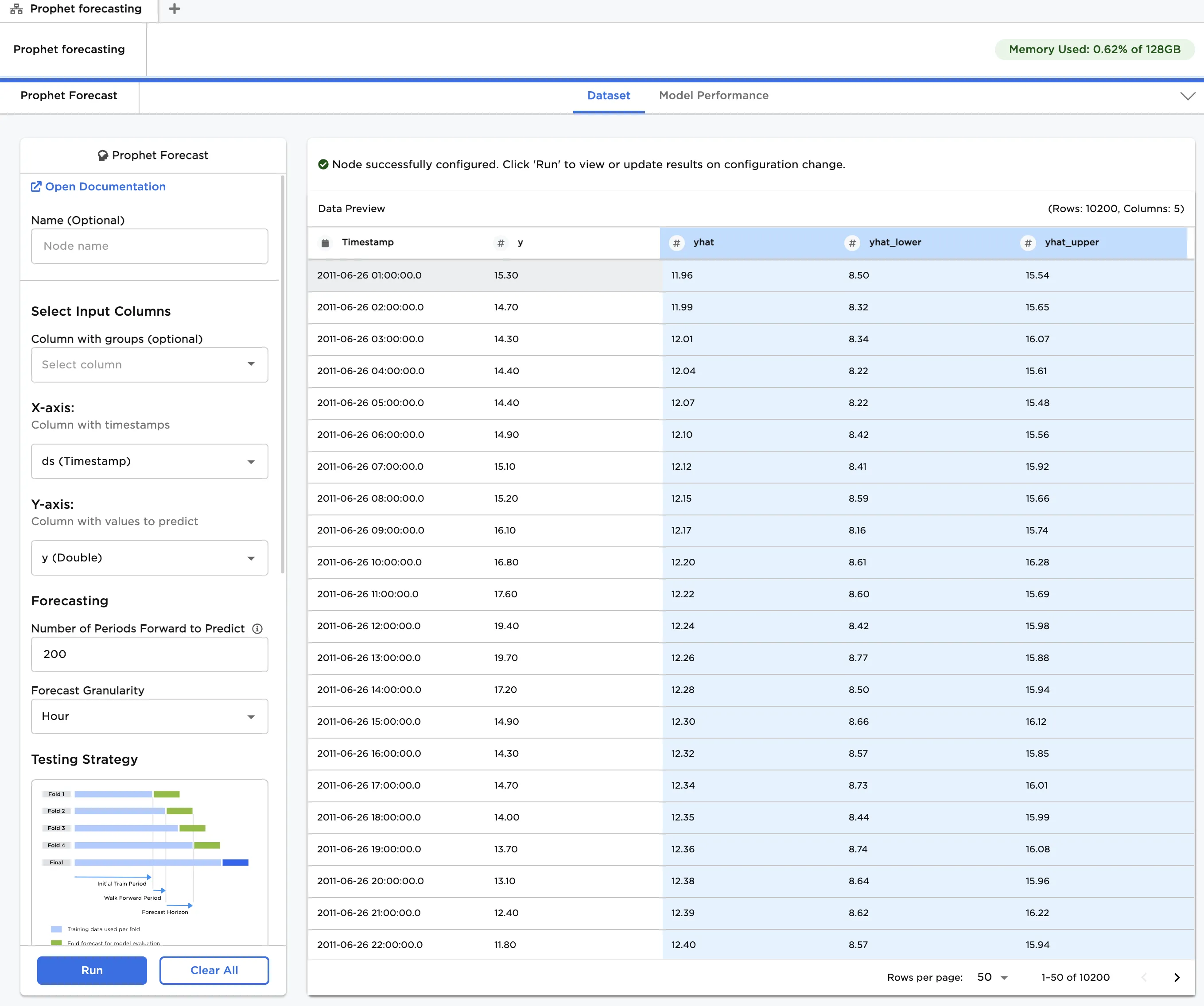
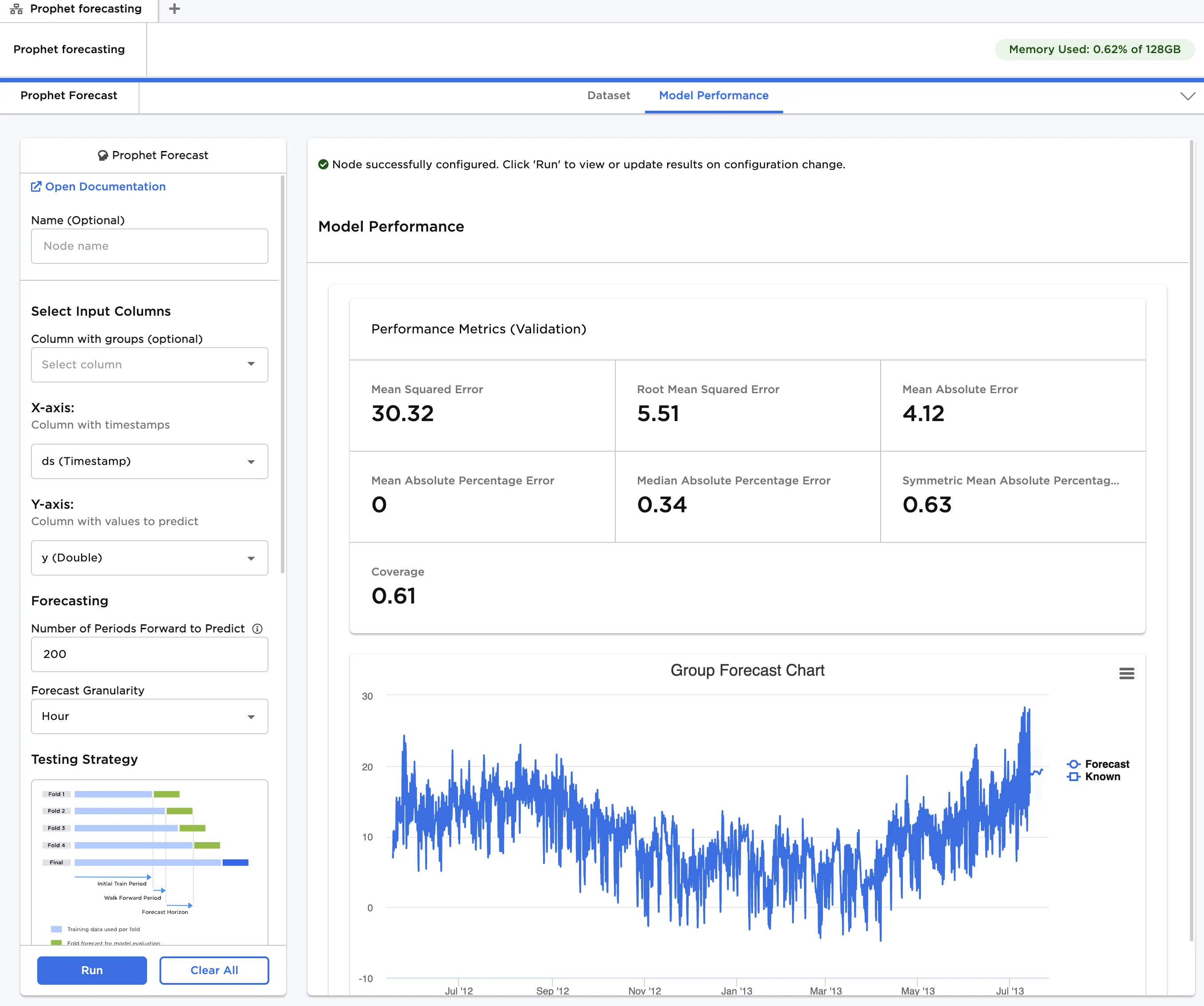
Figure 1: Example output
Examples
The dataframe shown in Figure 2 contains hourly temperature data from January, 1990 to April, 1992 in Cork, Ireland. Since the data experiences strong seasonal effects, and includes several seasons of history, we expect Prophet to work well in forecasting the temperature. For clarity, this is a univariate forecasting problem because we are modeling a single variable, temperature, over time, and using only its prior values to predict future values. Prophet can also handle multivariate timeseries, which have multiple time-dependent variables that can influence the variable to predict.
The Prophet model provides a suite of advanced configuration capabilities to improve data modeling and forecast accuracy. In this example, we will leverage basic functionality to generate a forecast.
Click here to learn more about Prophet.
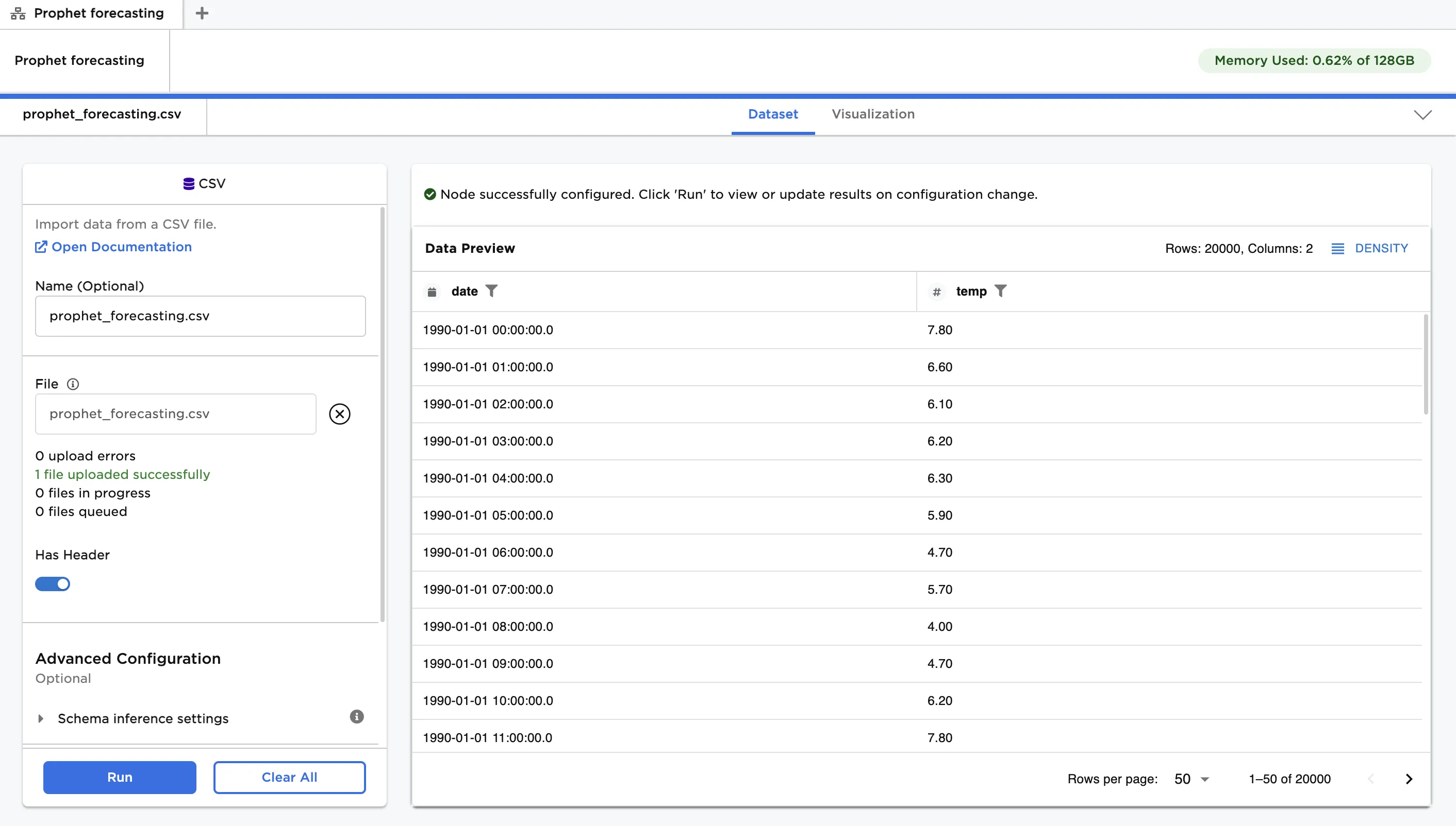
Figure 2: Example input data
Follow the steps below to fit a model of the input data and generate a forecast.
- Connect a Prophet node to an existing node.
- Select date (Timestamp) for the X-axis field and temp (double) for the Y-axis field.
- Set the Number of Periods Forwards to Predict to 14 days.
- Set the Initial Training Period to 400 days, the Walk Forward Period to 30 days, and the Forecast Horizon to 14 days. Since we are dealing with temperature data in a specific location, a period of at least 365 days, or 1 year, should adequately capture any trend and seasonality. This is the justification for setting the initial training period to 400 days. The forecast horizon is the same as the out-of-sample forecast period specified in Step 2. The intuition here is that performing cross-validation and predictions under the same conditions allows us to correctly identify the set of hyperparameters which result in the best forecast performance. With a 400-day initial training period, 833 days worth of data (i.e., from 01/01/1990 to 04/13/1992), and a 30-day walk forward period, we can expect 14 SHFs. This provides an adequate number of observations for cross-validation without significantly increasing computational effort. The number of SHFs can be determined using the following equation:
Here, $\Delta t_h$ is the period of all input training data, $\Delta t_{ITP}$ is the Initial Training Period and $\Delta t_{WFP}$ is the Walk Forward Period.
The cross-validation model performance, based on hyperparamer settings in Advanced Configuration, is displayed using several metrics. This includes Mean Squared Error, Root Mean Squared Error, Mean Absolute Error, Mean Absolute Percentage Error, Median Absolute Percentage Error, Symmetric Mean Absolute Percentage Error and Coverage.
Note in our example, the Mean Absolute Percentage Error (MAPE) is 0, not because the model has perfect performance, but because several temperature values are equal to zero. This means their percentage error relative to the forecast is undefined, causing Visual Notebooks to skip the calculation.
If the model doesn't perform as well as you'd like it to, try altering the advanced configuration options and training new models.
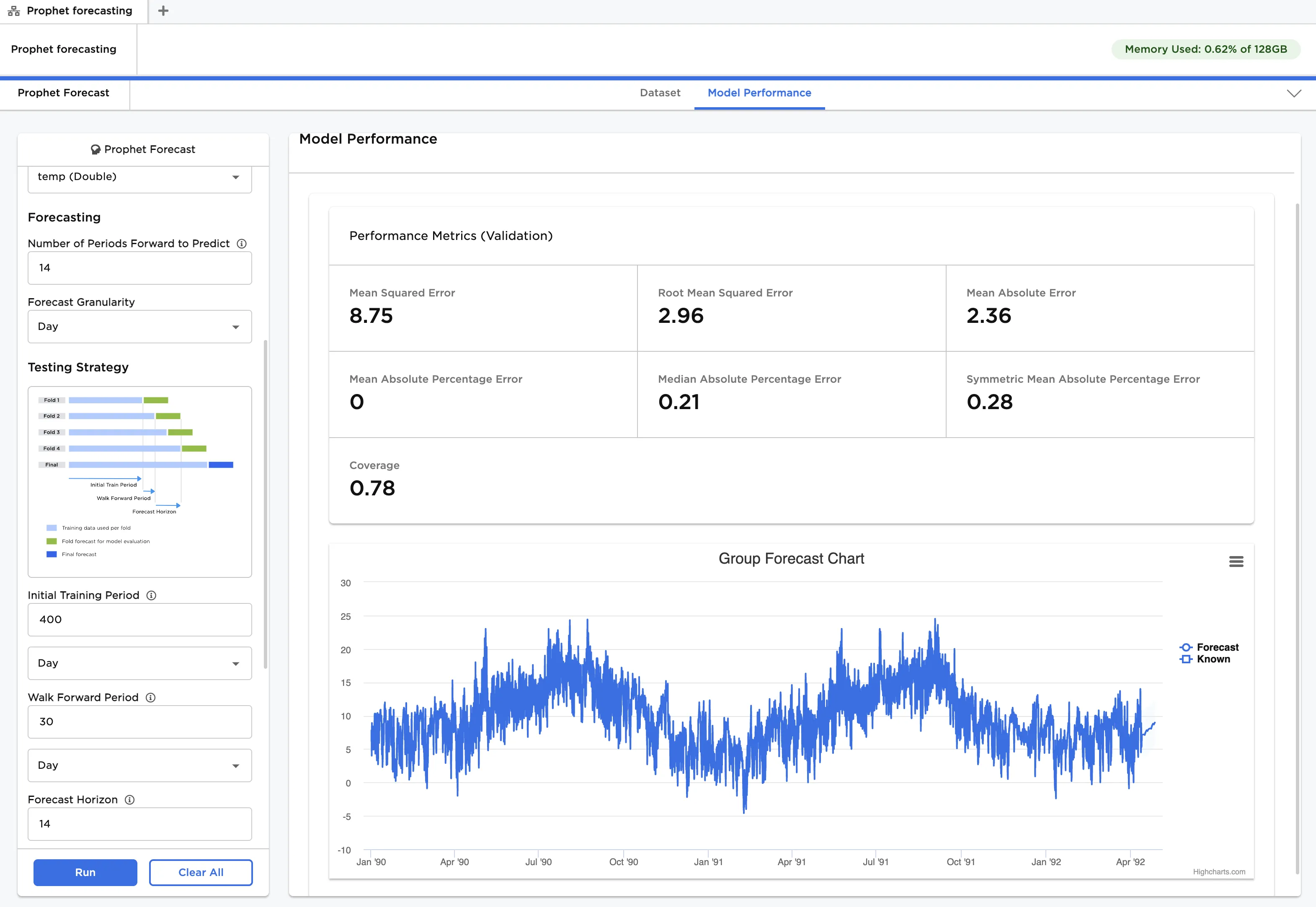
Figure 3: Model performance
To view the 14-day out-of-sample forecast more closely, click Forecast in the chart legend. The blue line with markers shows the forecasted values, and the highlighted region shows the uncertainty interval, whose bounds are indicated in the range.
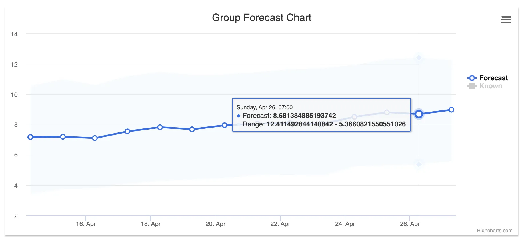
Figure 4: Forecast chart
Navigate to the Dataset tab to view the model's predictions. You will see values for both the historical data and the out-of-sample forecast. Input temperature values are labeled y, and predicted values are labeled yhat, with yhat_lower and yhat_upper defining the uncertainty interval.
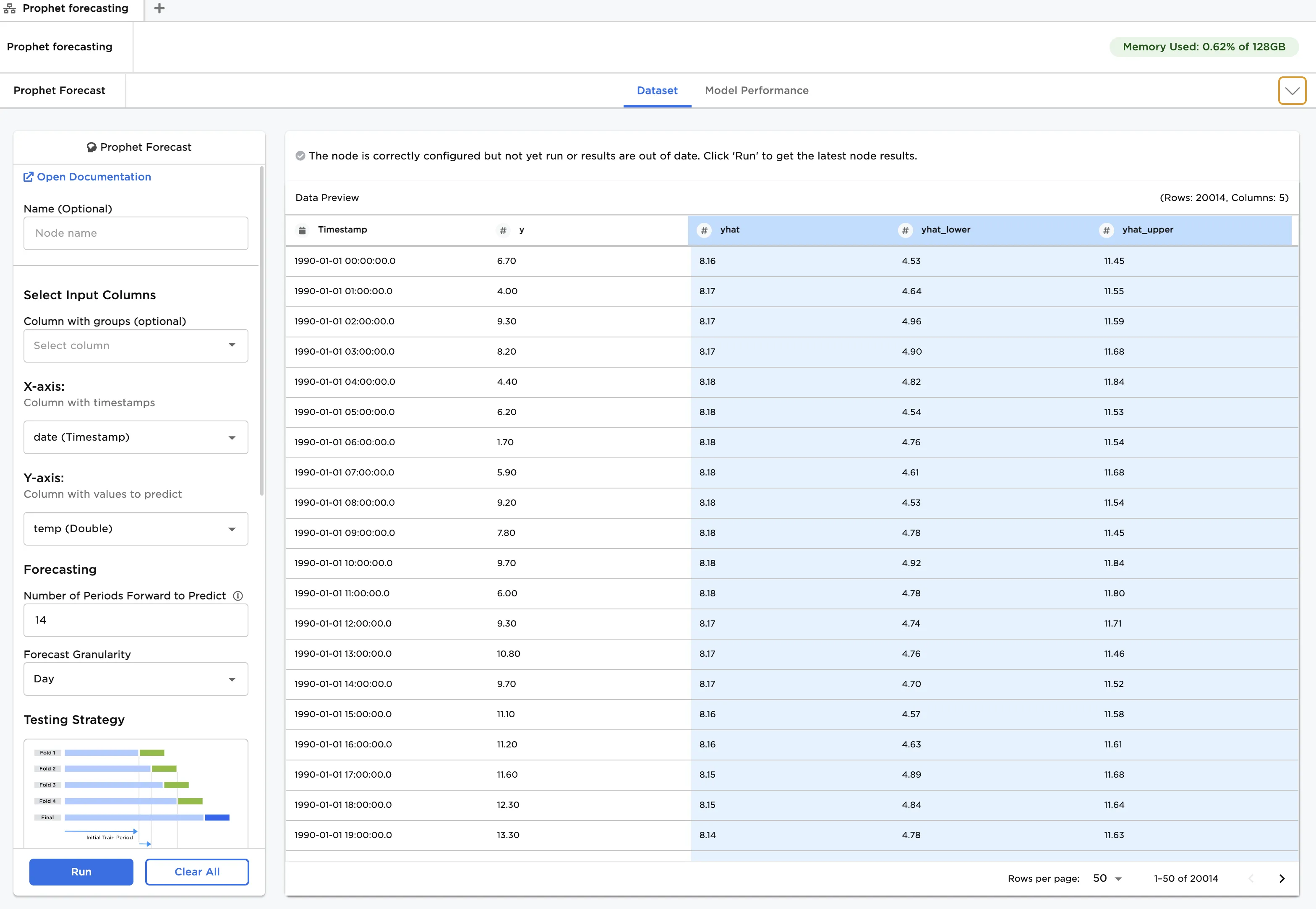
Figure 5: The selected model's predictions
To view the out-of-sample forecast, sort the Timestamp column in descending order by hovering over the column label and clicking the arrow that appears. Note the yhat values where y vales are NaN.
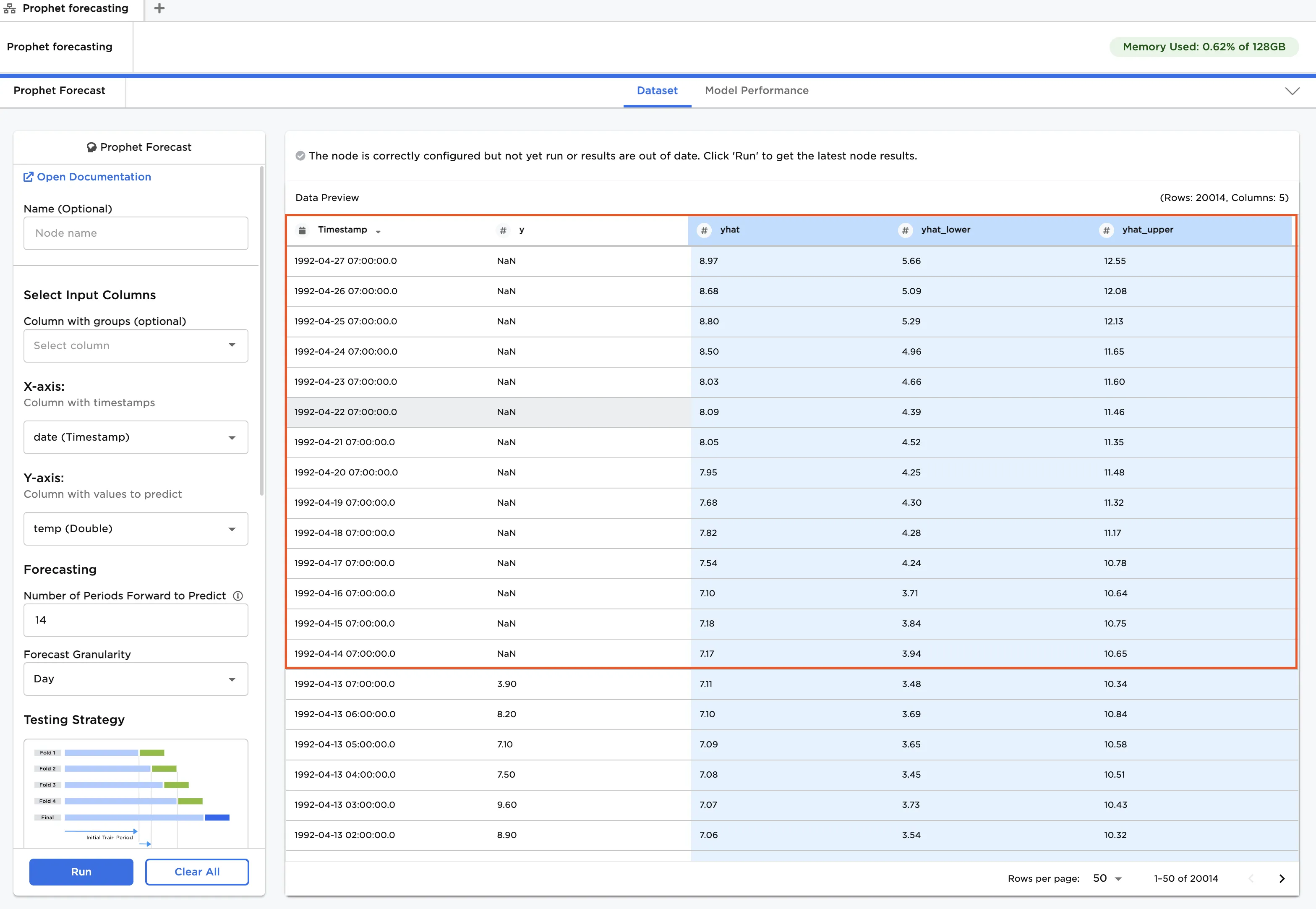
Figure 6: Forecast data