Rolling Cumulative Aggregate
The Rolling Cumulative Aggregate node in Visual Notebooks calculates rolling and cumulative functions over time such as average, sum, difference, maximum, minimum, median, standard deviation, and variance for columns with integers and doubles.
Configuration
| Field | Description |
|---|---|
| Name | Field to name the node An optional user-specified node name displayed in the workspace, both on the node and in the dataframe as a tab. |
| Time Column | Column to use in the calculation Select a column that contains timestamp (or numeric data) from the dataset to use in the calculation. |
| Group by | Grouping selection Select whether to view the data in a single series or grouped by data in another column. |
| Select column to partition with | Column to group by If Group data by column is selected for the Group by field, select a column to partition the data. |
| Feature Creation | Create the functions for the feature Make selections for the Select Window Columns() and Select Function(s) dropdown menus. Multiple features can be added. |
| Select Window Column(s) | Select column(s) to view rolling cumulative aggregate calculations Select columns with data to analyze the rolling cumulative aggregate over time. Multiple columns can be selected at once. |
| Select Function(s) | Select the calculation Select the calculations for the rolling cumulative aggregate. Choose between: average, sum, difference, maximum, minimum, median, standard deviation, and variance. Multiple functions can be selected at once. |
Node Inputs/Outputs
| Input | A dataframe in Visual Notebooks |
|---|---|
| Output | ** A dataframe with results of the Rolling Cumulative Aggregate selections** |
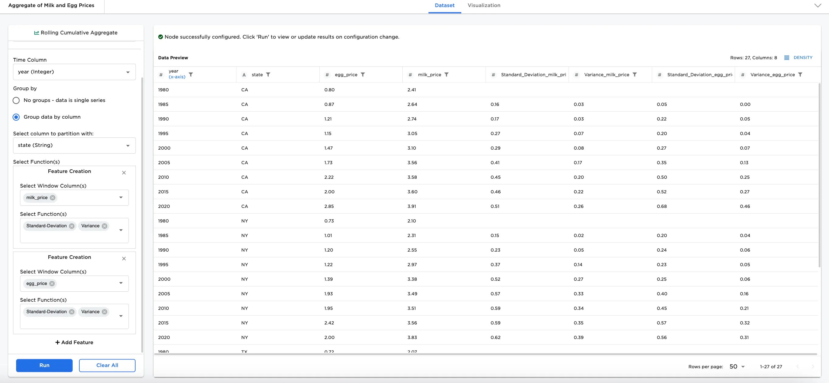
Figure 1: Example output
Examples
At times, it can be useful for businesses with new product ideas to analyze prices related to goods over time. Let's say your company has a product dependent on milk and egg markets and you want to analyze and compare the average, maximum, minimum, standard-deviation, and variance of the price of milk and eggs over time from one state to another. The dataframe shown in Figure 2 contains data about the price of milk and eggs in three US states from 1980 to 2020.
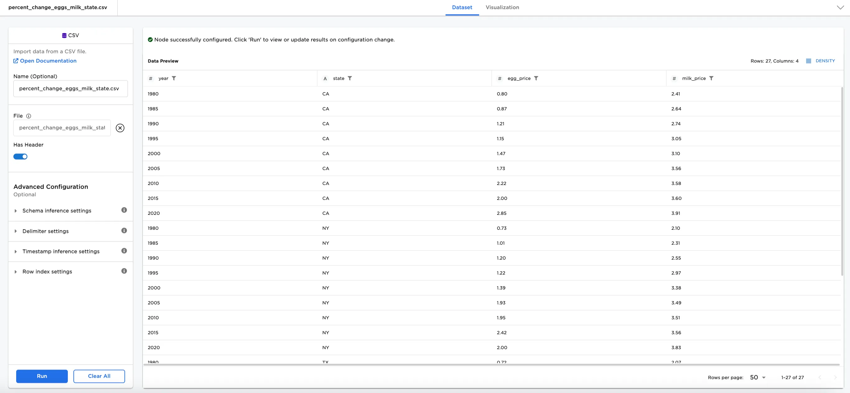
Figure 2. Example input data
The following are definitions for important rolling cumulative aggregate fields used in this node:
- Time Column field: A timestamp column is ideal to calculate the rolling cumulative aggregate over time periods, but if your data does not have a timestamp column, selecting another column with another ordering system (month 1, month 2, for example) also works. If a numeric data field is selected, Visual Notebooks orders the data in the field in sequence (values are represented from lowest to highest).
- Select Function(s) field: Select a function or multiple functions to apply on the columns selected in the Select Window Column(s) dropdown menu. Each selection creates a new column that combines the function name with the columns selected in Select Window Column(s). For example, selecting
Averageandegg_pricecreates a new column called, "Average_egg_price." Multiple columns and multiple functions can be selected at once to create multiple new columns. For convenience and readability, separate feature selections can also be created.
- Connect a Rolling Cumulative Aggregate node to an existing node. In this case, it is connected to a CSV node with the "Eggs_Milk_State" file.
- Optionally, name the Rolling Cumulative Aggregate node. In the example, the node is named, "Aggregate of Milk and Egg Prices."
- Select the Column with Timestamps or Sequence (x axis) field. Figure 3 shows
year (integer)selected for this field. - Make your Feature Creation selections. In the example,
milk_priceis selected for the Select Window Column(s) field, andAverage,Maximum,Minimum,Standard-DeviationandVarianceare selected for the Select Function(s) field.
Notice Figure 3 includes several new columns combining each selected function with milk_price.
 Figure 3: Example of rolling cumulative aggregate functions on milk price
Next, group the data by state:
- Select Group data by column
- In the Select column to partition with dropdown menu, select
state (String).
Notice that the columns in Figure 4 are now grouped by the state column year over year.
Alternatively (not shown), year (Integer) can be selected in the Select column to partition with dropdown menu to see the same data grouped by the year column, state by state.
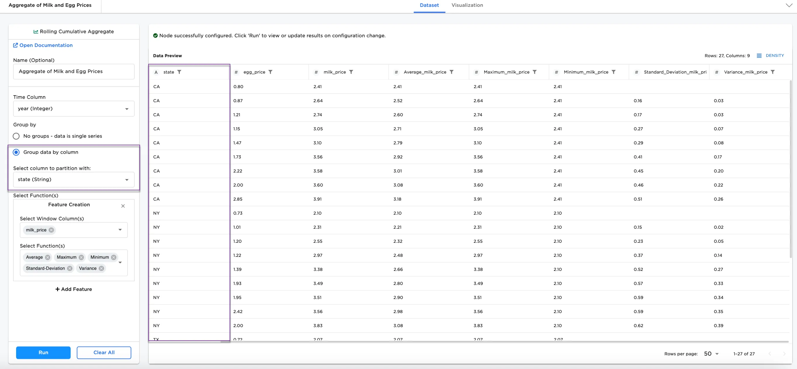 Figure 4: Example grouped by state
Optionally, you can add another column to view and compare rolling cumulative aggregate over time. In Figure 5, egg_price is added to the Select Window Column(s). Notice that new columns are created combining each function with egg_price.
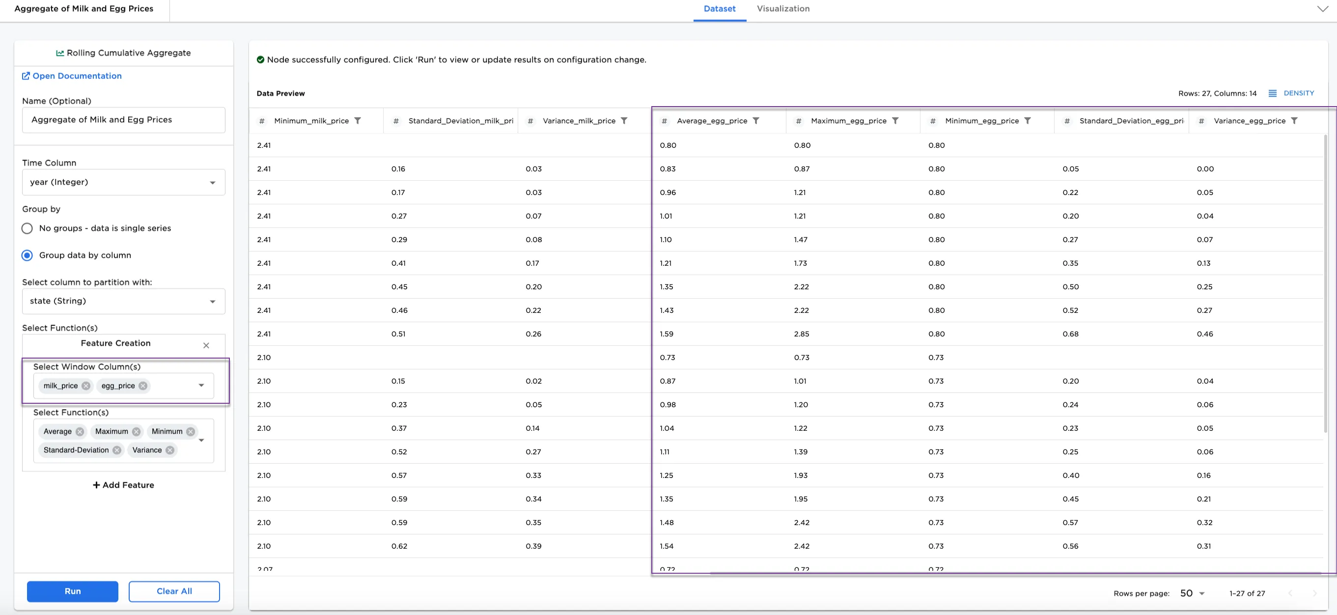
Figure 5: Example selecting two columns
To see a different way to use this node, try adding egg_price as an additional feature:
- Select + Add Feature
- Select Window Column(s):
egg_price(returning the original feature to onlymilk_price) - Select Function(s):
Standard-deviationandVariance
Notice that there are 4 columns showing Standard-deviation_milk_price, Variance_milk_price, Standard-deviation_egg_price, and Variance_egg_price.
Note: This is a similar result as having only one feature with both milk_price and egg_price in one Select Window Column(s) field. Both ways of adding features are available for your own datasets that could be more complex than the example dataset.
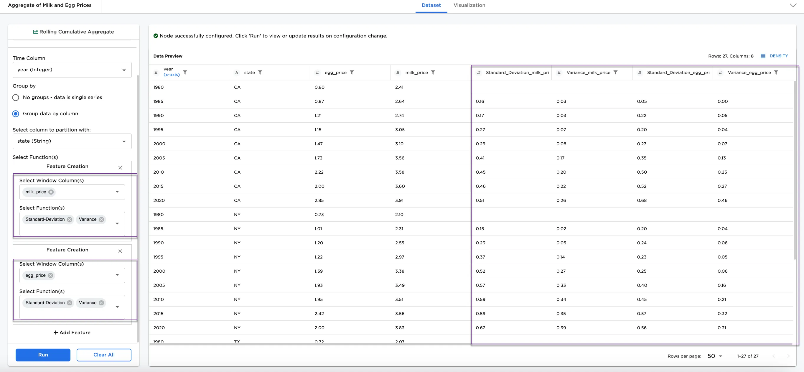
Figure 6: Example with multiple features