Source to Destination Path
Determine the shortest unweighted path between two nodes, using Visual Notebooks.
Configuration
| Field | Description |
|---|---|
| Name (Optional) | A user-specified node name displayed in the workspace |
| Source ID | id of first vertex Select the id of the first vertex of the path. |
| Destination ID | id of final vertex Select the id of the final vertex of the path. |
| Output Graph Format | Full output graph or computed path graph Choose to either generate a graph showing only the vertices needed (as well as their order) to traverse the shortest distance from the beginning point to the final point, or to generate a graph showing all of the points available in the space. |
| Vertex Order | Label for vertex order column Optionally specify a custom label for the column showing vertex order. |
| Vertex Along Path | Label for vertex along path column Optionally specify a label for the column showing whether that vertex is part of the shortest computed path. A value of 0 indicates that the vertex is part of the path, while a value of 1 indicates that the vertex is not part of the path. |
| Edge Order | Label for edge order column Optionally specify a custom label for the column showing edge order. |
| Edge Along Path | Label for Edge Along Path column Optionally specify a label for the column showing whether that edge is part of the shortest computed path. A value of 0 indicates that the edge is part of the path, while a value of 1 indicates that the edge is not part of the path. |
Node Inputs/Outputs
| Input | A Visual Notebooks Assemble Graph node |
|---|---|
| Output | Tables showing the vertices and edges used in the shortest path between two user-specified nodes. |
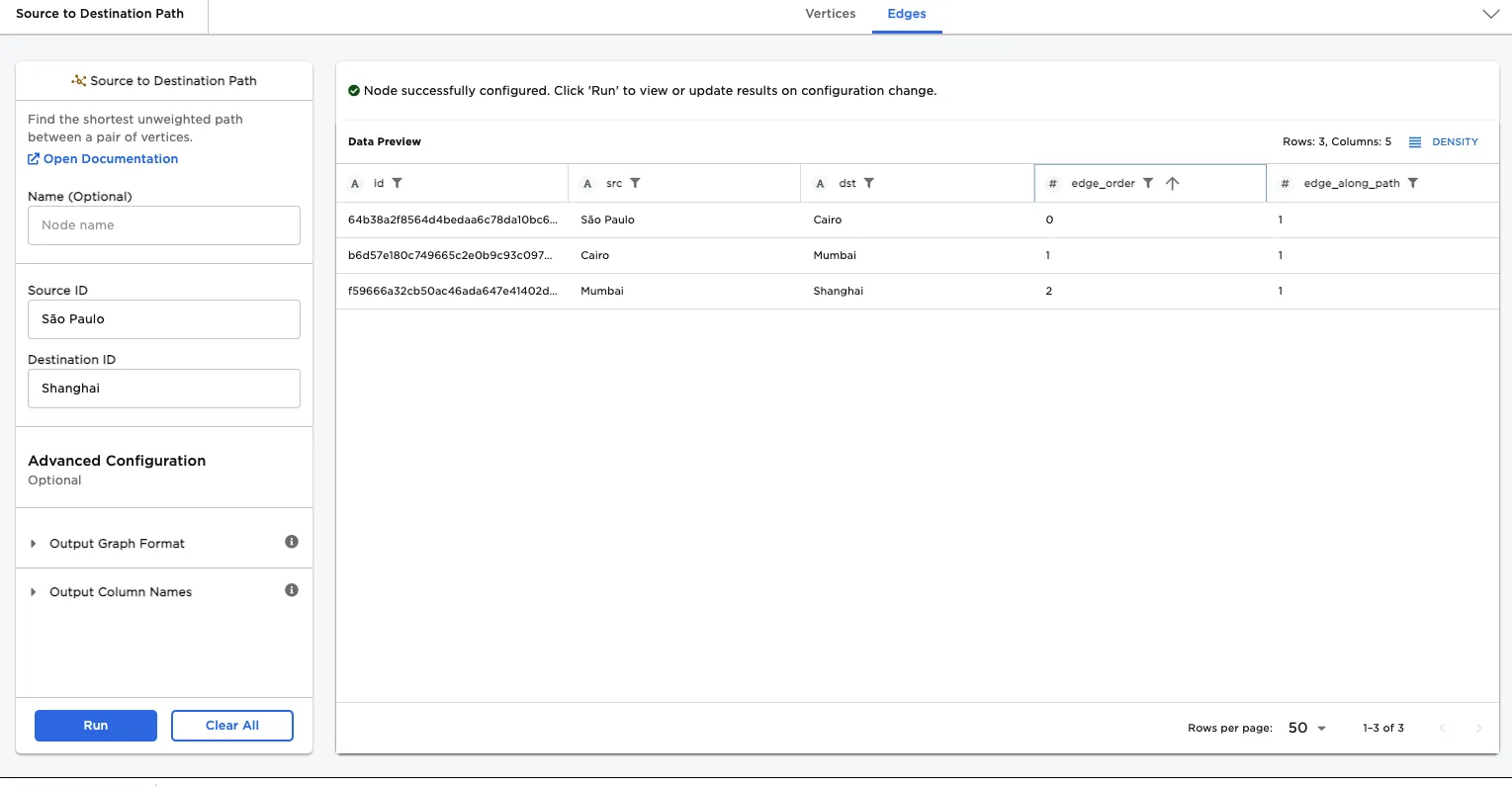
Figure 1: Example dataframe output
Examples
The Source to Destination Path node computes the shortest unweighted path between points, commonly referred to as vertices. The rules linking the vertices are in the form of edge data. Consider an airplane route that travels from Atlanta to NYC to Los Angeles, and then back to Atlanta. The vertices representing this path would be Atlanta, NYC, and Los Angeles. The edges would be Atlanta-NYC, NYC-Los Angeles, and Los Angeles-Atlanta.
To compute the shortest path between two vertices, the Source to Destination Path node requires both vertex and edge data. The vertices data and edge data used in the examples is shown in the following two images. The vertices data has one column, which shows a number of airport cities, and the edges data has two columns, one of which shows where a flight takes off from, and one of which shows where a flight lands.
For the first example, we will determine the shortest path from São Paulo to Shanghai. This requires three input nodes: two CSV nodes, and an Assemble Graph node, which are populated with data as follows:
- Import the data using CSV nodes. (See the documentation for the CSV node for additional details. Note that in general, you can import data to Visual Notebooks using other data integration nodes.)
- Connect each of the CSV nodes to an Assemble Graph node. (See the documentation for the Assemble Graph node for additional details.)
- Select Run.
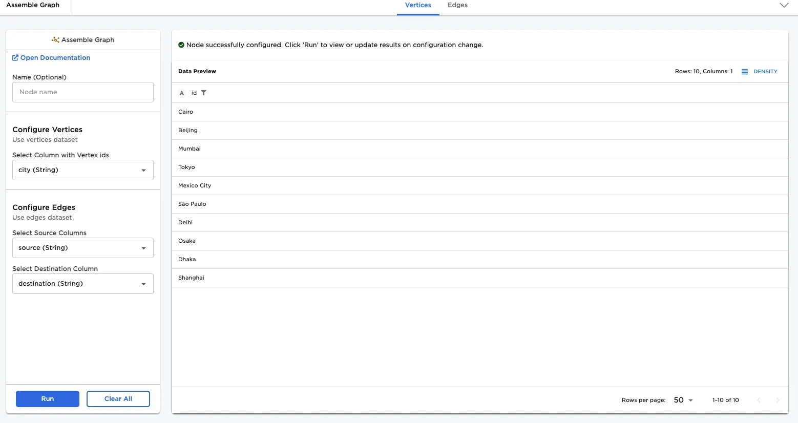
Figure 2: Example vertices input data
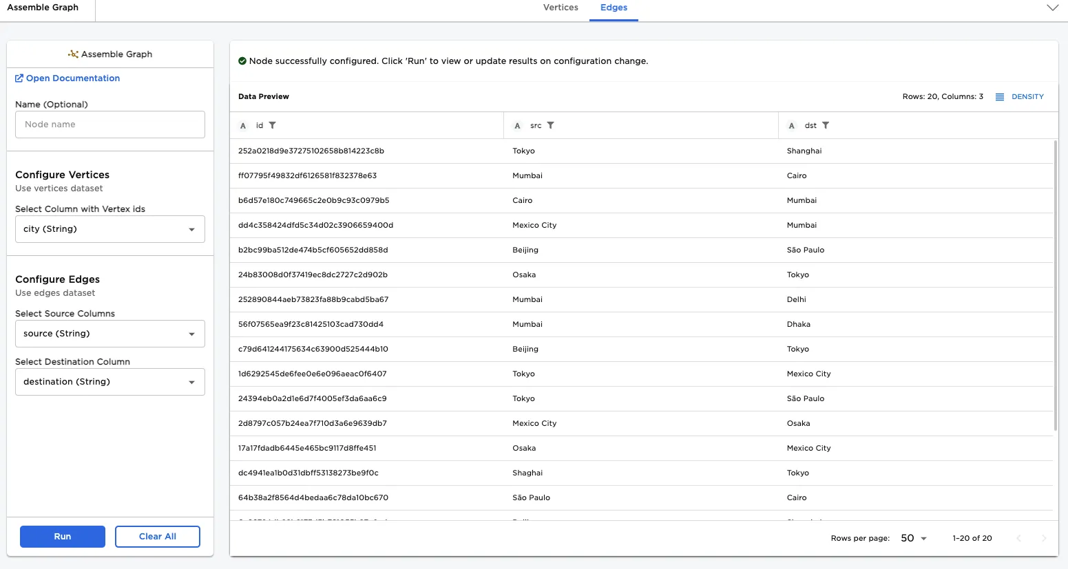
Figure 3: Example edges input data
To generate the path from São Paulo to Shanghai, do the following:
- Connect the Assemble Graph node to a Source to Destination Path node.
- For Source ID, enter "São Paulo".
- For Destination ID, enter "Shanghai".
- Select Run.
- After the output is generated, sort the vertex_order column in ascending order. Hover over the column name and select the arrow when it appears.
The output shows four vertices, in order from the starting point (São Paulo) to the final point (Shanghai).
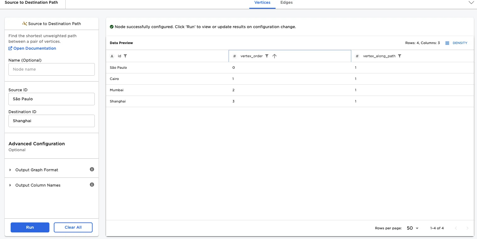
Figure 4: Shortest path from São Paulo to Shanghai
The Edges tab shows the exact same computed output, but in a slightly different form. Instead of showing individual points along the path, each segment of the path, in the form of a starting point and ending point, is shown. Since there were four points from start to end, there are three segments in the graph.
Figure 5: Shortest path from São Paulo to Shanghai, shown as edges
Optionally, to visualize the output, connect a Graph node, configure it, and select Run. (See the documentation for the Graph node for additional details on configuration. Note: These examples only use the Graph node to produce a visualization. The Graph node is not needed to use the Source to Destination Path node.)
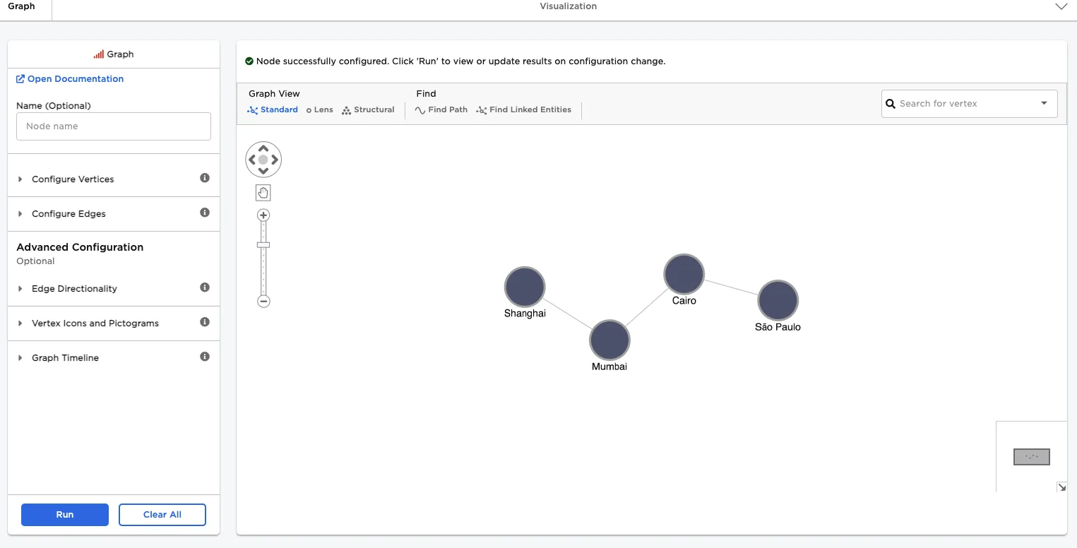
Figure 6: Graph of shortest path from São Paulo to Shanghai
To see the path in the context of all of the data points, instead of just the ones used in the path, do the following:
- From the Source to Destination Path node, select the Vertices tab.
- From the Output Graph Format section, select Return full input graph, with the shortest path vertices and edges labeled.
- Select Run.
- Hover over the label of the Edges column. When the arrow appears, select it to sort the column in ascending order.
- Scroll through the list to the bottom to see the edges of the graph from São Paulo to Shanghai.
All of the edges are now shown, instead of just the three edges needed to go from the origin to the destination. This context may be useful for considering alternate routes. Notice that cities that aren't part of the shortest path computed all have a value of -1 in the edge_order column.
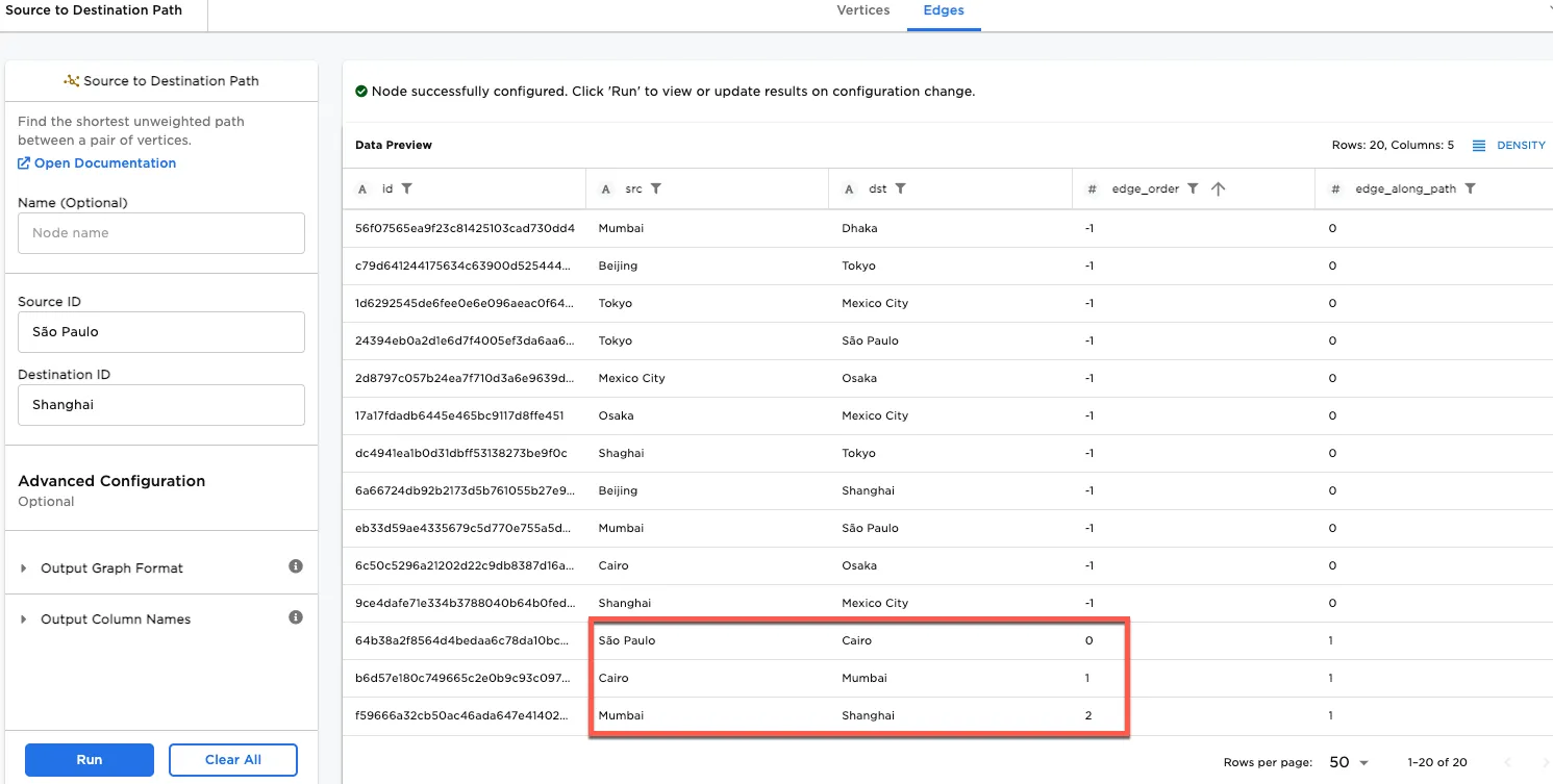
Figure 7: Full path from São Paulo to Shanghai
The full path, with all of the edges, can be visualized using a Graph node. The following figure shows this, where the shortest path from São Paulo to Shanghai has been highlighted. (Highlighting is not present in output of node.)
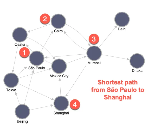
Figure 8: Graph of full path from São Paulo to Shanghai
For the final example, we will format the output to add custom column names, by doing the following:
- From the Source to Destination Path node, select the Vertices tab.
- From the Advanced Configuration Optional section, expand Output Column Names.
- For Vertex Order, specify Custom.
- After the screen refreshes, enter "Order".
- Select Run.
- Hover over the Order column name, and when an arrow appears, select it, to order the column in increasing order.
The output renders again, with one of the columns now labeled Order.
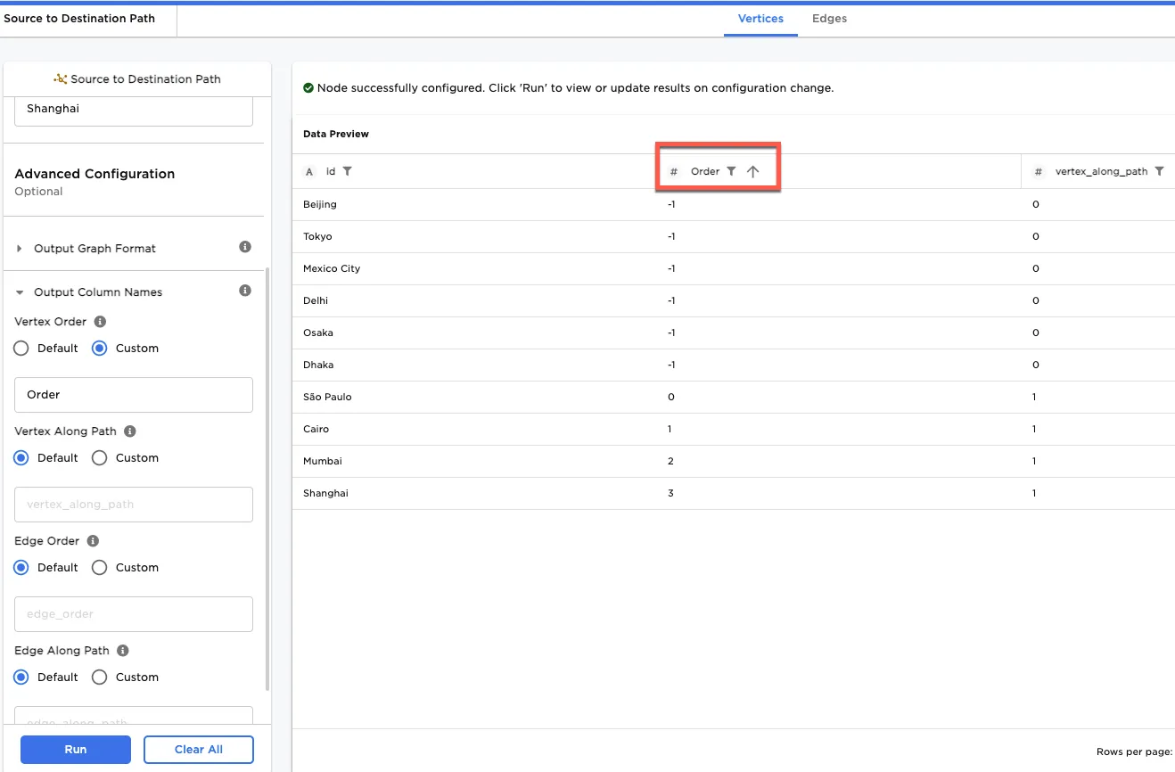
Figure 9: Custom column name