Simple Metrics
Simple metrics are instructions for how to produce a Timeseries object from any stream of data that represents a time series.
Simple metrics can produce four categories of Timeseries objects: continuous numeric, continuous enumerated, discontinuous point events, and discontinuous interval events.
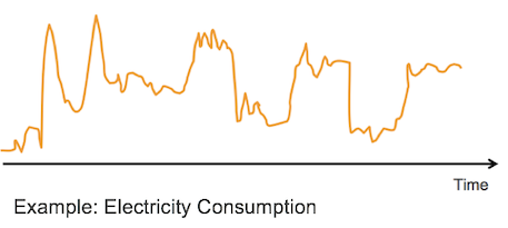 | Continuous numeric has a standard time interval that can report a data point. The data point could be body temperature, heart rate, electricity consumption, etc. |
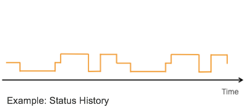 | Continuous enumerated is similar to continuous numeric, except there is an enumerated, or itemized list of values each time is associated with, rather than any kind of specific numeric value. This can be a history of statuses, for example when a device was on or off. |
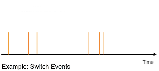 | Discontinuous point events occur at any point in time and do not have a standard time interval. For example, a light bulb is switched on at 12:05 PM, and it's switched off at 12:15 PM. |
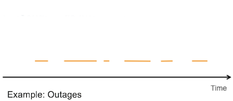 | Discontinuous interval events can occur at any point in time, but they are time bound. For example, an outage occurred from 3:03 PM to 3:05 PM. |
Core fields
Simple metrics are instances of the SimpleMetric Type. Here are the key fields to specify when declaring a SimpleMetric Type:
id(string) —idis inherited from the Persistable Type. The naming convention of the Simple Metricidfield should adhere to the following format:name_srcType. For example,AveragePower_SmartBulbshould be theidof a metric that can output a Timeseries of the average power of a SmartBulb. These should be global and unique.name(string) — Thenameshould be the descriptor of what the metric does. For example, AveragePower could be the name of a metric which can report the average power series of a SmartBulb. The convention here is CamelCase.srcType(string) — Entity for which to analyze data.path(string) — Thepathfield is the path from thesrcTypeto the Type where the metric data gets evaluated. For cases where evaluation needs to happen on the same Type, do not specify the path. This can be timed-dependent if any of the following Types are in it:- TimedValue or any Type that mixes it (TimedRelation, TimedCharacteristic)
- TimedIntervalValue or any Type that mixes it (TimedIntervalRelation, TimedIntervalCharacteristic)
expression(string) — Theexpressionfield is the expression that must be evaluated on the Type the path leads to. This is configured using the Expression Engine Function library.- Non-normalizable data
- Constant function:
expression: "identity(1)" - Piecewise constant function with aggregation across space:
expression: "sum(length)" - Binary function:
expression: "manufacturer == 'A'" - Ternary condition function:
expression: "job == 'B' ? 1: 0" - String function:
expression: "startsWith(model, 'X')"
- Constant function:
- Normalizable data
- Continuous numeric function with aggregation across space and time:
expression: "avg(avg(normalized.data.power))". Normalized keyword is not an actual field, it indicates that the metric engine should use normalized data
- Continuous numeric function with aggregation across space and time:
tsDecl,actionDeclare optional fields that may be used in place of expression
- Non-normalizable data
Expression details
Aggregating over time and space
For normalizable data, the expression can look to aggregate across space and time. Consider the expression defined below:
expression: "avg(avg(normalized.data.power))"
In the provided example, you can see two fields: data and power, which are linked together. It is important to note that these fields belong to different Types. In effect, these fields indicate a path saying to the effect of: go to the field data on a certain Type, which can then lead to another Type that has a field named power, that contains the data for analysis.
Assume the data for power is coming from two different sensors on the same light bulb. It is also measured at irregular frequencies, as shown in the image below in step (1).
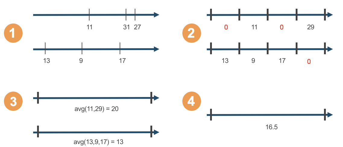
Next, consider the expression normalizing that data. This is indicated by the keyword normalized (normalized.data.power). For more information about the keyword normalized, see Normalization Engine. In this example, the normalization interval is set to be a quarter hour with default zero interpolation and the default average treatment.
What this means is there should be one value for every 15 min interval which can be calculated using an average aggregation. In step (2) the two readings within the last interval for the first sensor were averaged, producing a value of 29. Additionally, note that in intervals for which there was no value, the normalization process placed a 0 – this is a zero interpolation.
The third step is inner aggregation, aggregation over time. The expression calls for an average as the aggregation method over time: (avg(normalized.data.power)) Assuming the interval for evaluation of the metric is specified as HOUR (meaning 1 value for each hour interval). The resulting data is averaged as shown.
When the average is taken, the 0 points that were interpolated are not included. This is because the C3 Agentic AI Platform knows that these values are 100% made up, and so they are not counted.
You can opt for these made up values to be considered by calling a method called fillMissing.
The final fourth step is the outer aggregation, which is aggregation across space (or sources). (avg(avg(normalized.data.power))). This aggregates all separate Timeseries into a single Timeseries by averaging them, as seen in the example above.
Path details
There are three main steps in determining the path:
- Choose the source. The source is the Type on which to evaluate the metric. The SmartBulb Type is the source for evaluating the AveragePower metric.
- Determine where to locate the data. For AveragePower, it is defined as the field on the Type SmartBulbMeasurement.
- Figure out how to get from the source to the field that contains the data you need to analyze.
In determining the path, it is helpful to consider the data model, reproduced for this example below:
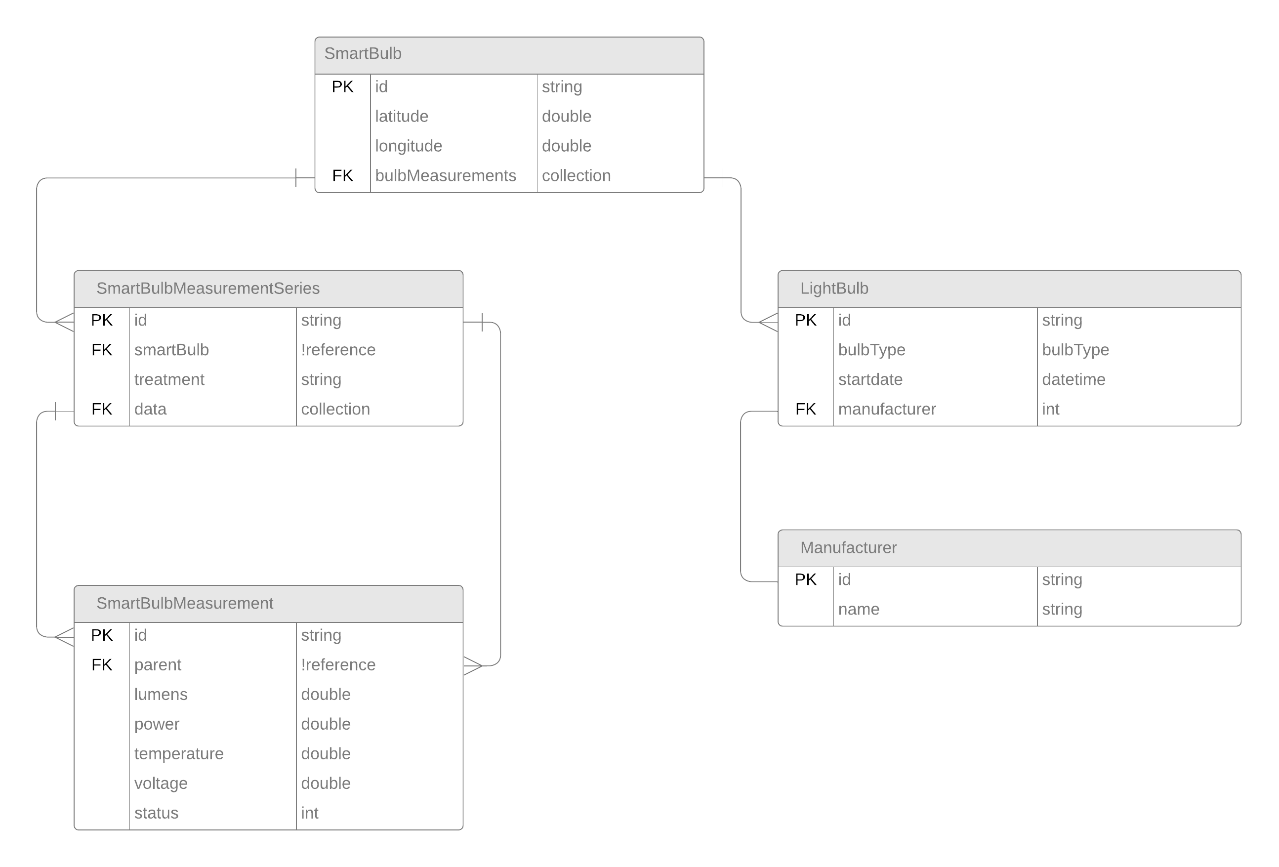
The SmartBulb Type contains a field called bulbMeasurements, which connects to the SmartBulbMeasurementSeries Type. The SmartBulbMeasurementSeries Type serves as the timeseries header Type.
Inside the SmartBulbMeasurementSeries Type, the data field points to the SmartBulbMeasurement Type. The SmartBulbMeasurement Type is where you can find the power field, which holds the data for analysis.
To locate the power field, follow this path:
SmartBulb → bulbMeasurements → data → power
Here is the step-by-step process:
- Start with the
bulbMeasurementsfield in theSmartBulbType. This field links to theSmartBulbMeasurementSeriesType, which organizes the time series data. - From the
SmartBulbMeasurementSeriesType, use thedatafield to reach theSmartBulbMeasurementType, which contains individual data points. - Finally, access the
powerfield in theSmartBulbMeasurementType to retrieve the data needed for analysis.
Important observations to note:
- The path
bulbMeasurementsgets you from the source Type to the header Type. - The expression
data.powergets you from the header Type to the data (field) you want to analyze. The expression also dictates the logic to apply on the data:(avg(avg(normalized.data.power)))
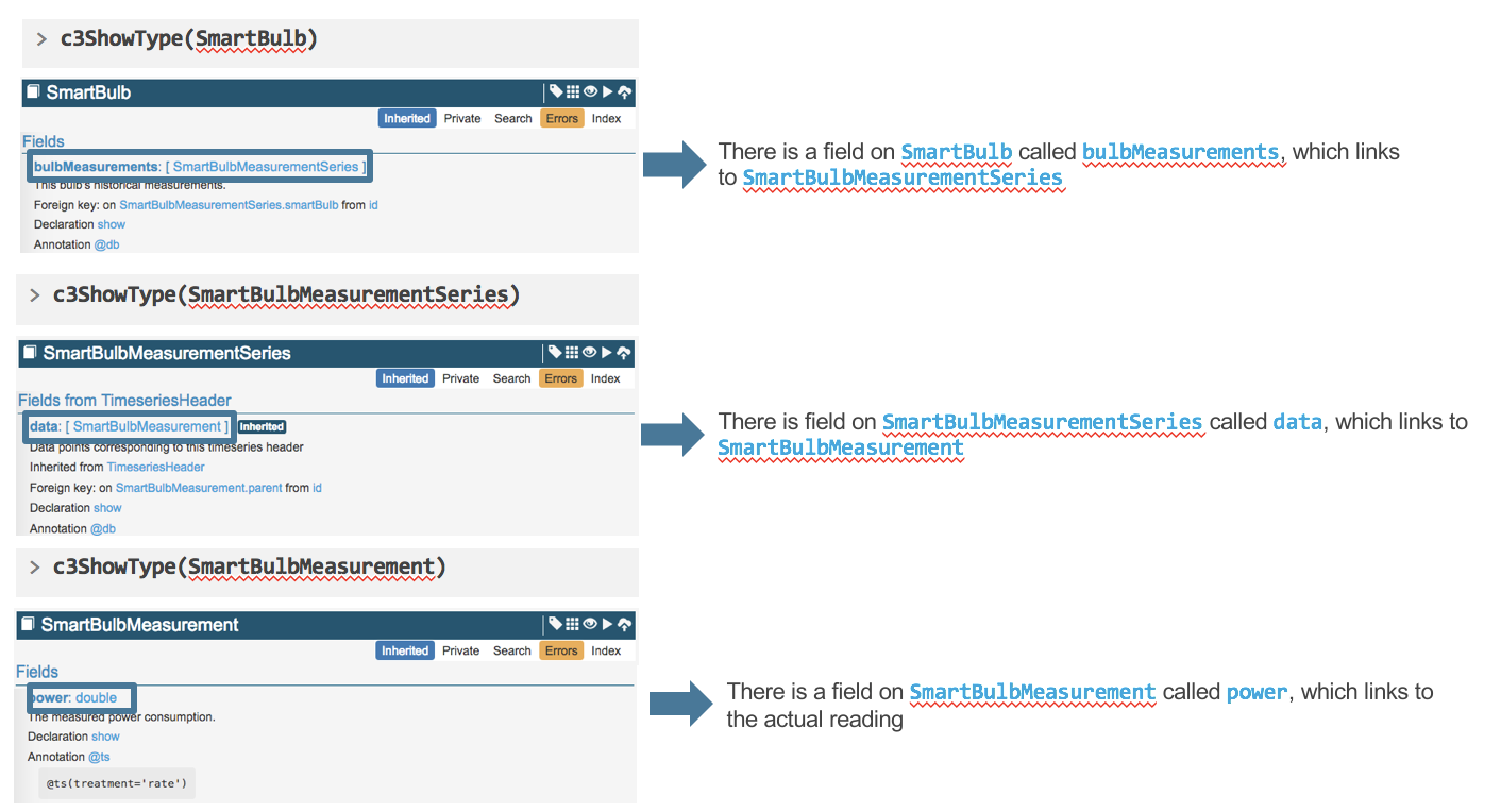
Retracing the path
The path of information from source Type to data can be accessed by looking at the Type documentation. Begin at the source and select the link to the pertinent Type.
The example Simple Metric definitions for the categories continuous numeric and discontinuous interval events are below:
Continuous numeric
{
  "id": "AveragePower_SmartBulb",
  "name": "AveragePower",
  "srcType": "SmartBulb",
  "description": "Average power over time of the smart bulb",
  "path": "bulbMeasurements",
  "expression": "avg(avg(normalized.data.power))"
}Discontinuous interval events
{
  "id": "ManufacturerNameStartsWithG_SmartBulb",
  "name": "ManufacturerNameStartsWithG",
  "description": "True or false for duration of LightBulb",
  "srcType": "SmartBulb",
  "expression": "startsWith(lowerCase(manufacturer.name), 'g')"
}