Data Lakehouse Quickstart
This quickstart takes you from an empty Data Lakehouse to a table you can query, entirely in the browser. You upload a CSV in the Create new table wizard, run a SQL query in the SQL Editor, and view the run on the Spark Executions page. An alternative notebook path is included at the end for users who prefer code.
The scenario uses wind turbine measurements (active power, rotor speed, gear oil temperature) from a fictional utility, Atlas Power. The same pattern works for any tabular dataset.
Before you start
Complete the steps in Data Lakehouse Prerequisites. You also need a CSV file with wind turbine measurements; the header row must include the columns t, activePower, rotorSpeed, gearOilTemp, and asset.
Step 1: Open the Data Lakehouse page
- Open your application in C3 AI Studio.
- Select Data Lakehouse in the Data section of the side navigation.
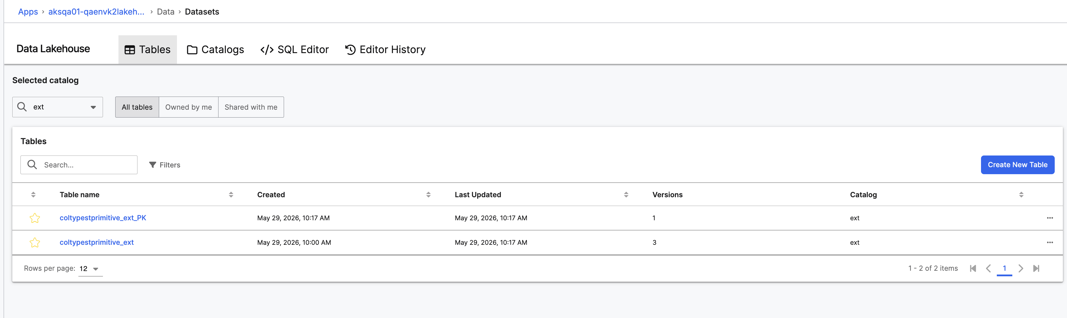
The page opens on the Tables tab.
Step 2: Create a table from your CSV
- On the Tables tab, select Owned by me.
- Select Create new table.
- Select Browse, and choose your CSV file.
- Verify the parsed information:
- Files: The file you uploaded is listed.
- Schema: Column names and inferred data types match the CSV header.
- Target preview: The first rows look correct.
- File settings: If the preview looks wrong, change the delimiter.
- Select Next.
- Enter
turbineMeasurementsas the Table name, and a short description. - Select Upload.
The wizard creates an Iceberg table in your default catalog and loads the CSV in one step.
Step 3: Inspect the table
- Select the SQL Editor tab.
- Set Catalog to your default catalog (
datasetsin most applications) and Namespace to the namespace that holds the new table. - In the View Reference Table panel, pick
turbineMeasurementsfrom the Select Table... combobox and select View Reference Table.
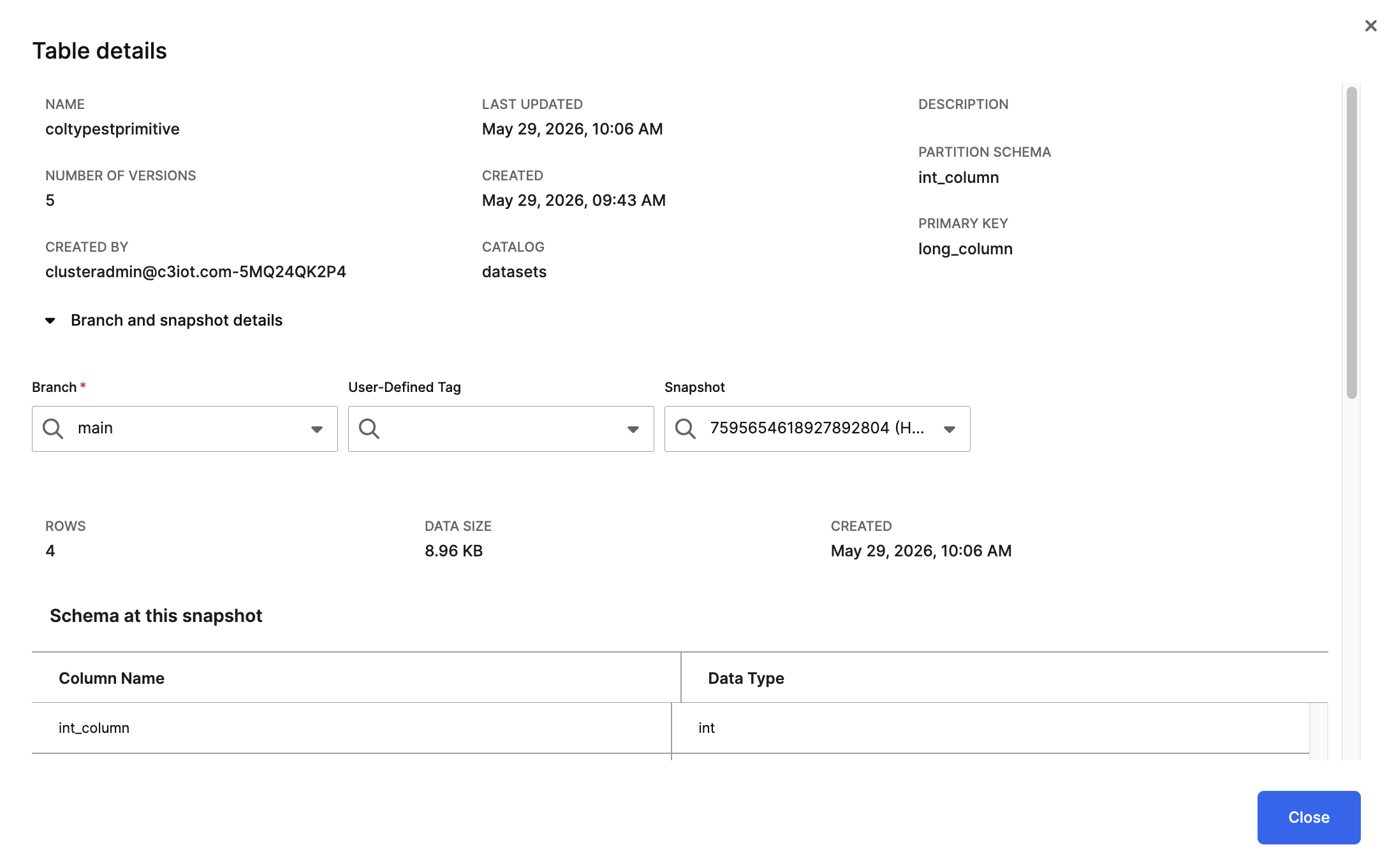
The Table details modal shows the schema, the current snapshot, the partition expressions, and a 20-row data preview.
Step 4: Run a SQL query
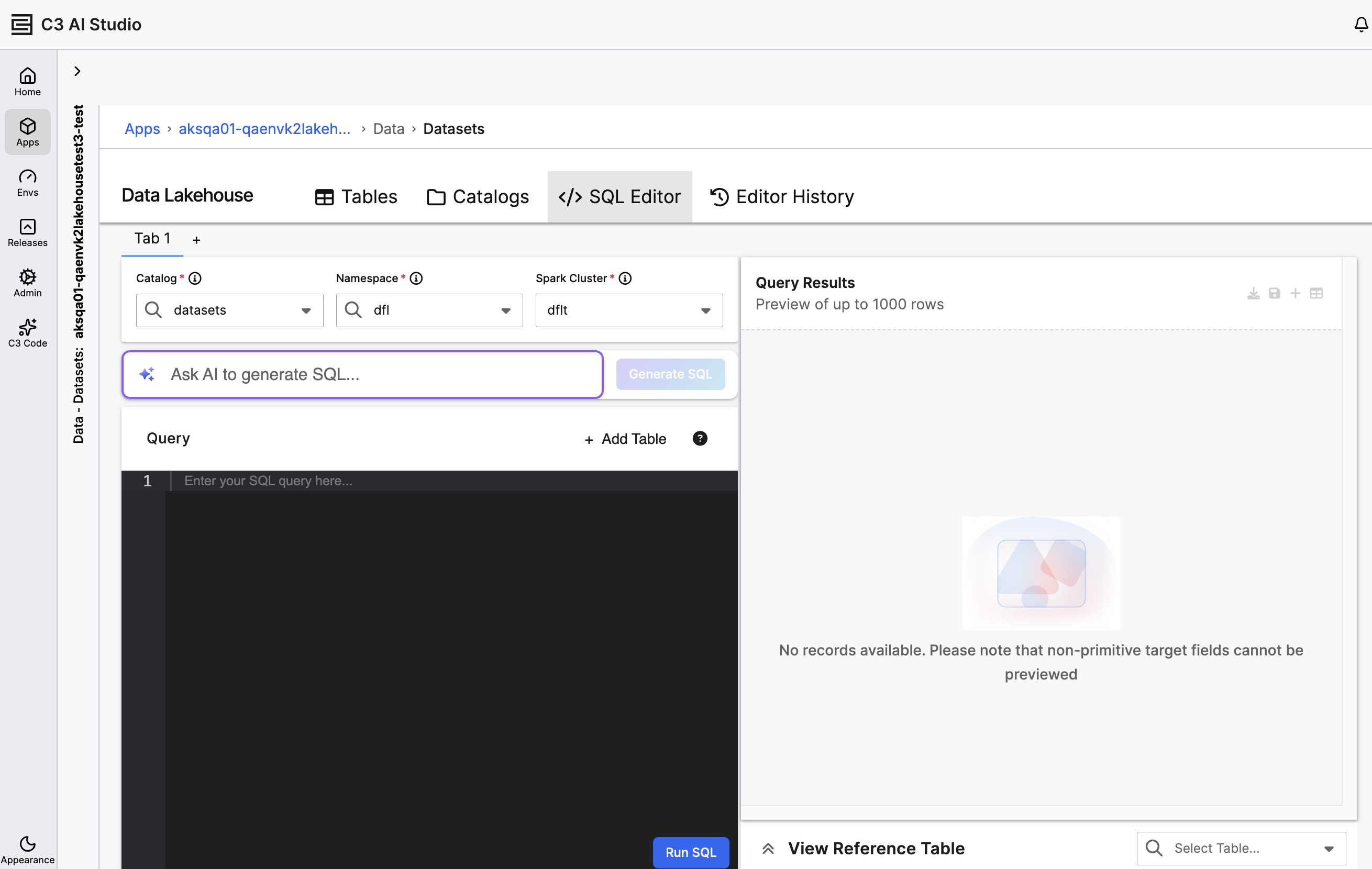
Close the Table details modal. In the SQL Editor query area, enter the following query and select Run SQL.
SELECT asset, AVG(activePower) AS avgPower
FROM turbineMeasurements
GROUP BY asset
ORDER BY avgPower DESC
LIMIT 10
Add a WHERE clause on t to restrict the aggregate to a specific time range (for example, WHERE t >= CURRENT_DATE - INTERVAL '1 YEAR'). Match the literal to the date range in your CSV.
If the cluster is hibernated, a banner appears: Starting Spark cluster, query response will be available shortly. The query queues until the cluster is Running. Cold start can take several minutes; subsequent queries against a warm cluster return in seconds.
The results pane shows the per-asset averages. Use the toolbar above the pane to download the result as CSV, save it as a new Lakehouse table, or switch to a chart view.
Step 5: Track the run on the Spark Executions page
- In the side navigation, expand Jobs.
- Select Spark Executions.
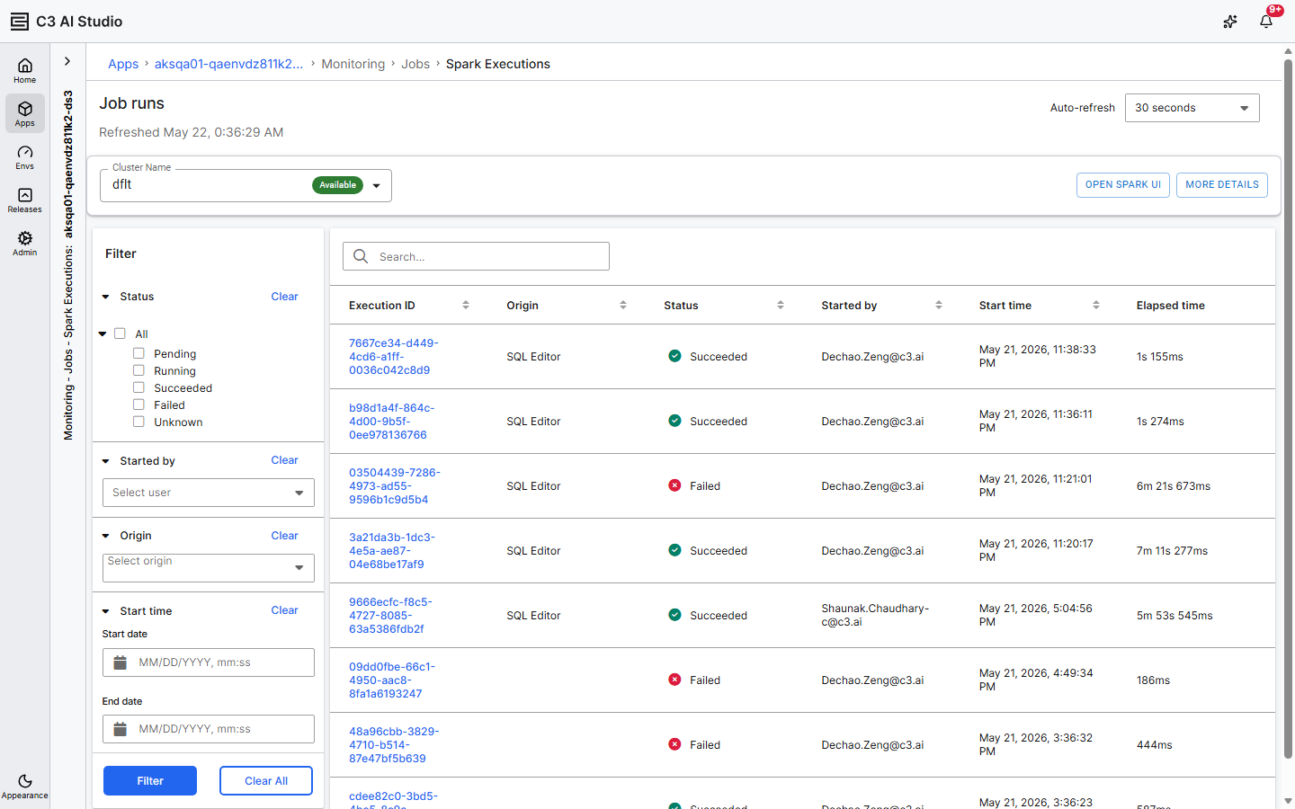
Your query appears as a SparkExecution row with Origin = SQL Editor. The SparkExecutionOrigin enum defines two values in 8.11: SQL Editor and Source to DataLake. Select the execution ID to open the detail drawer with the catalog, namespace, query text, and error message (if any).
What you built
You now have:
- An Iceberg table in your default catalog with the data from your CSV file.
- A SQL query that runs against the table and produces an aggregate.
- A record of the query on the Spark Executions page, with a link back to the cluster log.
Alternative: run the same flow from a notebook
If you prefer code, the same steps run from a Jupyter notebook or the Studio Console. The notebook path also lets you set primary keys, custom partitions, and sort orders that the Create new table wizard does not expose.
# 1. Start the cluster and get the default catalog
# This example assumes a Spark cluster named dedicated_spark exists. Replace the name with your cluster.
cluster = c3.SparkCluster.forName("dedicated_spark")
cluster.ensureService(waitForReady=True)
ss = cluster.dataSparkSession()
catalog = c3.DataLake.Catalog.inst()

# 2. Create the table with a primary key and partitions
schema = c3.ValueType.fromString(
    "{t: datetime, activePower: double, rotorSpeed: double, "
    "gearOilTemp: double, asset: string}"
)
spec = (
    c3.DataLake.CreateTableSpec.builder()
    .name("turbineMeasurements")
    .schema(schema)
    .partitionExpressions(["asset", "month(t)"])
    .primaryKeys(["asset", "t"])
    .build()
)
table = catalog.createTable(spec)

# 3. Load from CSV
table.importCsv(
    "gcs://atlas-power-sample/turbineMeasurements.csv",
    "append",
    c3.CsvParsingSpec.builder().header(True).build(),
)
importCsv accepts a cluster-accessible URL (gcs://, s3://, or azure://) — not a local file path on your workstation. The Create new table wizard (Step 2) hides this by uploading your browser file to the cluster before calling importCsv.
The dataSparkSession() call returns a Data.SparkSession, the C3 Agentic AI Platform's Pandas-on-Spark session with C3 helpers. The notebook write appears on the same Spark Executions page as a SparkExecution row.
For richer table creation, see Create and Load Data Lakehouse Tables.
Next steps
- To register a catalog other than the default Hadoop catalog, see Register a Data Lakehouse Catalog.
- To define more complex tables with custom partitions and merge semantics, see Create and Load Data Lakehouse Tables.
- To run analytical queries from a notebook with Pandas-on-Spark, see Transform Data Lakehouse Data with Spark.